![]()
Pandas functions for Time Series data
- Date Time Index
- Time Resampling
- Time Shifting
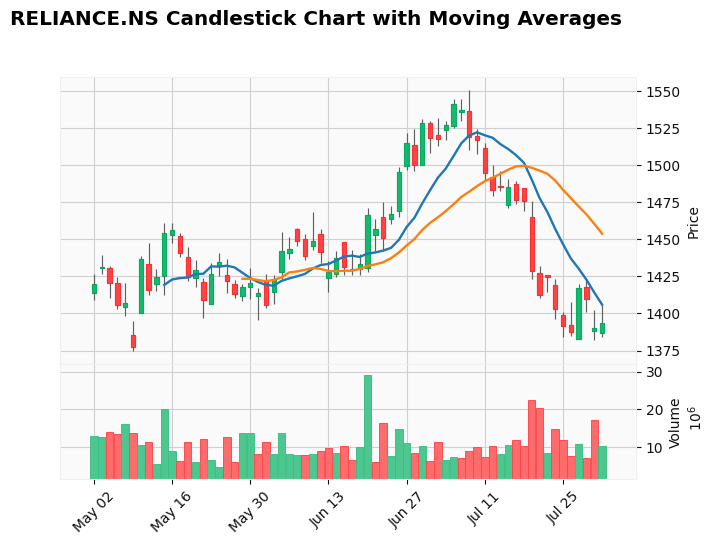
- Simple Moving Average (Rolling)
- Expanding
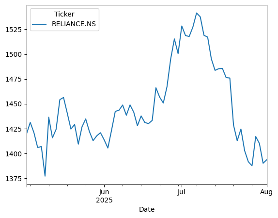
- Plotting
Date Time Index
['04/07/2025', '05/07/2025', '06/07/2025']DatetimeIndex(['2025-07-04', '2025-07-05', '2025-07-06'], dtype='datetime64[ns]', freq=None)--------------------------------------------------------------------------- NameError Traceback (most recent call last) /tmp/ipython-input-3468975073.py in <cell line: 0>() ----> 1 datetime.strptime('31/01/22 23:59:59.999999','%d/%m/%y %H:%M:%S.%f') NameError: name 'datetime' is not defined
Downloading...
From: https://drive.google.com/uc?id=1ugXf9514sOZx5izMY7Mt6_HX8doCQLcO
To: /content/Preprocessing3.csv
100%|██████████| 919k/919k [00:00<00:00, 78.0MB/s]'Preprocessing3.csv'| Date | Year | Locality | Estimated Value | Sale Price | Property | Residential | num_rooms | num_bathrooms | carpet_area | property_tax_rate | Face | |
|---|---|---|---|---|---|---|---|---|---|---|---|---|
| 0 | 2009-01-02 | 2009 | Greenwich | NaN | 5187000.0 | ? | Detached House | 3 | 2 | 1026.0 | 1.025953 | South |
| 1 | 2009-01-02 | 2009 | Norwalk | NaN | 480000.0 | Single Family | Detached House | 3 | 2 | 1051.0 | 1.025953 | West |
| 2 | 2009-01-02 | 2009 | Waterbury | 57890.0 | 152000.0 | Single Family | Detached House | 3 | 2 | 943.0 | 1.025953 | East |
| 3 | 2009-01-02 | 2009 | NaN | 44520.0 | 60000.0 | Single Family | Detached House | 3 | 2 | 1099.0 | 1.025953 | North |
| 4 | 2009-01-03 | 2009 | Bridgeport | 91071.0 | 250000.0 | Two Family | Duplex | 4 | 2 | 1213.0 | 1.025953 | South |
<class 'pandas.core.frame.DataFrame'>
RangeIndex: 10000 entries, 0 to 9999
Data columns (total 12 columns):
 #   Column             Non-Null Count  Dtype
---  ------             --------------  -----
 0   Date               10000 non-null  object
 1   Year               10000 non-null  int64
 2   Locality           8715 non-null   object
 3   Estimated Value    8719 non-null   float64
 4   Sale Price         10000 non-null  float64
 5   Property           10000 non-null  object
 6   Residential        10000 non-null  object
 7   num_rooms          10000 non-null  int64
 8   num_bathrooms      10000 non-null  int64
 9   carpet_area        8718 non-null   float64
 10  property_tax_rate  10000 non-null  float64
 11  Face               10000 non-null  object
dtypes: float64(4), int64(3), object(5)
memory usage: 937.6+ KBtake date feature and extract day month year from that
| Date | |
|---|---|
| 0 | 2009-01-02 |
| 1 | 2009-01-02 |
| 2 | 2009-01-02 |
| 3 | 2009-01-02 |
| 4 | 2009-01-03 |
<class 'pandas.core.frame.DataFrame'>
RangeIndex: 10000 entries, 0 to 9999
Data columns (total 1 columns):
 #   Column  Non-Null Count  Dtype
---  ------  --------------  -----
 0   Date    10000 non-null  datetime64[ns]
dtypes: datetime64[ns](1)
memory usage: 78.3 KB| Date | day | month | year | |
|---|---|---|---|---|
| 0 | 2009-01-02 | 2 | 1 | 2009 |
| 1 | 2009-01-02 | 2 | 1 | 2009 |
| 2 | 2009-01-02 | 2 | 1 | 2009 |
| 3 | 2009-01-02 | 2 | 1 | 2009 |
| 4 | 2009-01-03 | 3 | 1 | 2009 |
| ... | ... | ... | ... | ... |
| 9995 | 2022-09-30 | 30 | 9 | 2022 |
| 9996 | 2022-09-30 | 30 | 9 | 2022 |
| 9997 | 2022-09-30 | 30 | 9 | 2022 |
| 9998 | 2022-09-30 | 30 | 9 | 2022 |
| 9999 | 2022-09-30 | 30 | 9 | 2022 |
10000 rows × 4 columns
<class 'pandas.core.frame.DataFrame'>
RangeIndex: 144 entries, 0 to 143
Data columns (total 2 columns):
 #   Column                   Non-Null Count  Dtype
---  ------                   --------------  -----
 0   Month                    144 non-null    datetime64[ns]
 1   Thousands of Passengers  144 non-null    int64
dtypes: datetime64[ns](1), int64(1)
memory usage: 2.4 KB/tmp/ipython-input-65770057.py:3: FutureWarning: YF.download() has changed argument auto_adjust default to True
stock_data = yf.download(ticker_symbol, start='2024-01-01', end='2025-08-01', interval="1d")
[*********************100%***********************] 1 of 1 completed| Price | Close | High | Low | Open | Volume |
|---|---|---|---|---|---|
| Ticker | RELIANCE.NS | RELIANCE.NS | RELIANCE.NS | RELIANCE.NS | RELIANCE.NS |
| Date | |||||
| 2024-01-01 | 1290.744263 | 1299.016237 | 1282.223134 | 1285.910692 | 4030540 |
| 2024-01-02 | 1301.432983 | 1303.077427 | 1282.148458 | 1288.128164 | 7448800 |
| 2024-01-03 | 1287.281006 | 1312.545235 | 1284.241274 | 1300.585825 | 9037536 |
| 2024-01-04 | 1293.933350 | 1300.511122 | 1285.188128 | 1289.623028 | 9612778 |
| 2024-01-05 | 1299.439697 | 1305.494222 | 1294.606127 | 1297.047791 | 8086406 |
| ... | ... | ... | ... | ... | ... |
| 2025-07-25 | 1391.699951 | 1401.000000 | 1384.099976 | 1398.900024 | 11854722 |
| 2025-07-28 | 1387.599976 | 1407.800049 | 1385.000000 | 1392.300049 | 7748361 |
| 2025-07-29 | 1417.099976 | 1420.199951 | 1383.000000 | 1383.000000 | 10750072 |
| 2025-07-30 | 1410.099976 | 1423.300049 | 1401.300049 | 1418.099976 | 7209849 |
| 2025-07-31 | 1390.199951 | 1402.599976 | 1382.199951 | 1388.099976 | 17065827 |
392 rows × 5 columns
/tmp/ipython-input-1785857247.py:3: FutureWarning:

YF.download() has changed argument auto_adjust default to True

[*********************100%***********************] 1 of 1 completed| Price | Close | High | Low | Open | Volume |
|---|---|---|---|---|---|
| Ticker | RELIANCE.NS | RELIANCE.NS | RELIANCE.NS | RELIANCE.NS | RELIANCE.NS |
| Date | |||||
| 2025-05-02 | 1419.800049 | 1426.699951 | 1409.099976 | 1414.000000 | 13007841 |
| 2025-05-05 | 1431.300049 | 1439.500000 | 1426.900024 | 1431.000000 | 12685649 |
| 2025-05-06 | 1420.900024 | 1432.000000 | 1410.599976 | 1431.000000 | 14084117 |
| 2025-05-07 | 1406.000000 | 1424.400024 | 1402.699951 | 1420.900024 | 13440169 |
| 2025-05-08 | 1407.000000 | 1420.800049 | 1398.000000 | 1404.099976 | 16106175 |
| ... | ... | ... | ... | ... | ... |
| 2025-07-28 | 1387.599976 | 1407.800049 | 1385.000000 | 1392.300049 | 7748361 |
| 2025-07-29 | 1417.099976 | 1420.199951 | 1383.000000 | 1383.000000 | 10750072 |
| 2025-07-30 | 1410.099976 | 1423.300049 | 1401.300049 | 1418.099976 | 7209849 |
| 2025-07-31 | 1390.199951 | 1402.599976 | 1382.199951 | 1388.099976 | 17065827 |
| 2025-08-01 | 1393.699951 | 1405.900024 | 1384.300049 | 1386.900024 | 10321171 |
66 rows × 5 columns
Collecting mplfinance

  Downloading mplfinance-0.12.10b0-py3-none-any.whl.metadata (19 kB)

Requirement already satisfied: matplotlib in /usr/local/lib/python3.11/dist-packages (from mplfinance) (3.10.0)

Requirement already satisfied: pandas in /usr/local/lib/python3.11/dist-packages (from mplfinance) (2.2.2)

Requirement already satisfied: contourpy>=1.0.1 in /usr/local/lib/python3.11/dist-packages (from matplotlib->mplfinance) (1.3.2)

Requirement already satisfied: cycler>=0.10 in /usr/local/lib/python3.11/dist-packages (from matplotlib->mplfinance) (0.12.1)

Requirement already satisfied: fonttools>=4.22.0 in /usr/local/lib/python3.11/dist-packages (from matplotlib->mplfinance) (4.59.0)

Requirement already satisfied: kiwisolver>=1.3.1 in /usr/local/lib/python3.11/dist-packages (from matplotlib->mplfinance) (1.4.8)

Requirement already satisfied: numpy>=1.23 in /usr/local/lib/python3.11/dist-packages (from matplotlib->mplfinance) (2.0.2)

Requirement already satisfied: packaging>=20.0 in /usr/local/lib/python3.11/dist-packages (from matplotlib->mplfinance) (25.0)

Requirement already satisfied: pillow>=8 in /usr/local/lib/python3.11/dist-packages (from matplotlib->mplfinance) (11.3.0)

Requirement already satisfied: pyparsing>=2.3.1 in /usr/local/lib/python3.11/dist-packages (from matplotlib->mplfinance) (3.2.3)

Requirement already satisfied: python-dateutil>=2.7 in /usr/local/lib/python3.11/dist-packages (from matplotlib->mplfinance) (2.9.0.post0)

Requirement already satisfied: pytz>=2020.1 in /usr/local/lib/python3.11/dist-packages (from pandas->mplfinance) (2025.2)

Requirement already satisfied: tzdata>=2022.7 in /usr/local/lib/python3.11/dist-packages (from pandas->mplfinance) (2025.2)

Requirement already satisfied: six>=1.5 in /usr/local/lib/python3.11/dist-packages (from python-dateutil>=2.7->matplotlib->mplfinance) (1.17.0)

Downloading mplfinance-0.12.10b0-py3-none-any.whl (75 kB)

   ━━━━━━━━━━━━━━━━━━━━━━━━━━━━━━━━━━━━━━━━ 75.0/75.0 kB 1.8 MB/s eta 0:00:00

Installing collected packages: mplfinance

Successfully installed mplfinance-0.12.10b0
/tmp/ipython-input-3328782981.py:7: FutureWarning:

YF.download() has changed argument auto_adjust default to True

[*********************100%***********************] 1 of 1 completed| Price | Close | High | Low | Open | Volume |
|---|---|---|---|---|---|
| Ticker | RELIANCE.NS | RELIANCE.NS | RELIANCE.NS | RELIANCE.NS | RELIANCE.NS |
| Date | |||||
| 2025-05-02 | 1419.800049 | 1426.699951 | 1409.099976 | 1414.000000 | 13007841 |
| 2025-05-05 | 1431.300049 | 1439.500000 | 1426.900024 | 1431.000000 | 12685649 |
| 2025-05-06 | 1420.900024 | 1432.000000 | 1410.599976 | 1431.000000 | 14084117 |
| 2025-05-07 | 1406.000000 | 1424.400024 | 1402.699951 | 1420.900024 | 13440169 |
| 2025-05-08 | 1407.000000 | 1420.800049 | 1398.000000 | 1404.099976 | 16106175 |
| ... | ... | ... | ... | ... | ... |
| 2025-07-28 | 1387.599976 | 1407.800049 | 1385.000000 | 1392.300049 | 7748361 |
| 2025-07-29 | 1417.099976 | 1420.199951 | 1383.000000 | 1383.000000 | 10750072 |
| 2025-07-30 | 1410.099976 | 1423.300049 | 1401.300049 | 1418.099976 | 7209849 |
| 2025-07-31 | 1390.199951 | 1402.599976 | 1382.199951 | 1388.099976 | 17065827 |
| 2025-08-01 | 1393.699951 | 1405.900024 | 1384.300049 | 1386.900024 | 10321171 |
66 rows × 5 columns
| 0 | ||
|---|---|---|
| Price | Ticker | |
| Close | RELIANCE.NS | 0 |
| High | RELIANCE.NS | 0 |
| Low | RELIANCE.NS | 0 |
| Open | RELIANCE.NS | 0 |
| Volume | RELIANCE.NS | 0 |
DatetimeIndex(['2025-05-02', '2025-05-05', '2025-05-06', '2025-05-07',
               '2025-05-08', '2025-05-09', '2025-05-12', '2025-05-13',
               '2025-05-14', '2025-05-15', '2025-05-16', '2025-05-19',
               '2025-05-20', '2025-05-21', '2025-05-22', '2025-05-23',
               '2025-05-26', '2025-05-27', '2025-05-28', '2025-05-29',
               '2025-05-30', '2025-06-02', '2025-06-03', '2025-06-04',
               '2025-06-05', '2025-06-06', '2025-06-09', '2025-06-10',
               '2025-06-11', '2025-06-12', '2025-06-13', '2025-06-16',
               '2025-06-17', '2025-06-18', '2025-06-19', '2025-06-20',
               '2025-06-23', '2025-06-24', '2025-06-25', '2025-06-26',
               '2025-06-27', '2025-06-30', '2025-07-01', '2025-07-02',
               '2025-07-03', '2025-07-04', '2025-07-07', '2025-07-08',
               '2025-07-09', '2025-07-10', '2025-07-11', '2025-07-14',
               '2025-07-15', '2025-07-16', '2025-07-17', '2025-07-18',
               '2025-07-21', '2025-07-22', '2025-07-23', '2025-07-24',
               '2025-07-25', '2025-07-28', '2025-07-29', '2025-07-30',
               '2025-07-31', '2025-08-01'],
dtype='datetime64[ns]', name='Date', freq=None)<class 'pandas.core.frame.DataFrame'>
DatetimeIndex: 66 entries, 2025-05-02 to 2025-08-01
Data columns (total 5 columns):
# Column Non-Null Count Dtype
--- ------ -------------- -----
0 (Close, RELIANCE.NS) 66 non-null float64
1 (High, RELIANCE.NS) 66 non-null float64
2 (Low, RELIANCE.NS) 66 non-null float64
3 (Open, RELIANCE.NS) 66 non-null float64
4 (Volume, RELIANCE.NS) 66 non-null int64
dtypes: float64(4), int64(1)
memory usage: 3.1 KB