![]()
Time Series Data It refers to data that is collected, recorded or observed over time in a sequential order.
Characteristics: - Chronological Order : Observations are ordered in time (D, W, M, Y, s, m ,h) - Sequential Dependency : The order of the data matters because previous values can influence or predict the future values.
- Temporal components : Trend, Seasonality, Cycle, noise
Time series Analysis: - statistical technique : meaningful insights about pattern and trends - forecasting
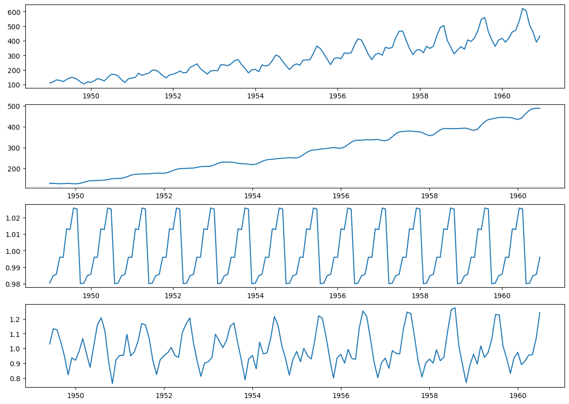
Time Series Decomposition - Trend : long term direction - Seasonality : repeting pattern at fixed interval - Noise
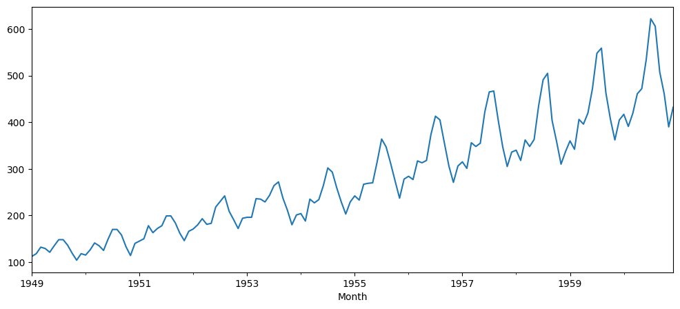
| Passengers | |
|---|---|
| Month | |
| 1949-01-01 | 112 |
| 1949-02-01 | 118 |
| 1949-03-01 | 132 |
| 1949-04-01 | 129 |
| 1949-05-01 | 121 |
| ... | ... |
| 1960-08-01 | 606 |
| 1960-09-01 | 508 |
| 1960-10-01 | 461 |
| 1960-11-01 | 390 |
| 1960-12-01 | 432 |
144 rows × 1 columns

- Additive $ y_t = T_t + S_t + R_t$
- Multiplicative $ y_t = T_t * S_t * R_t$
/tmp/ipython-input-979513816.py:3: FutureWarning: YF.download() has changed argument auto_adjust default to True
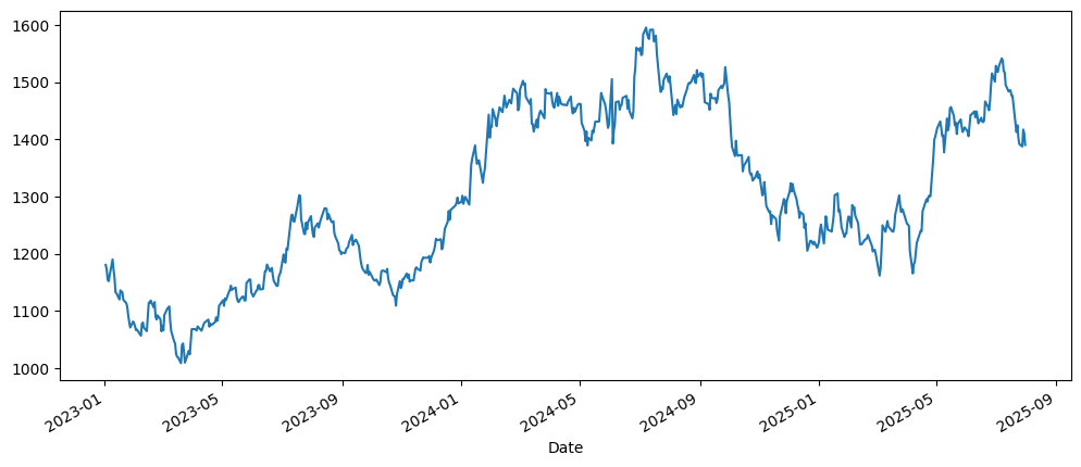
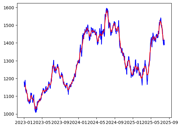
stock_data = yf.download(ticker_symbol, start='2023-01-01', end='2025-08-01', interval="1d")
[*********************100%***********************] 1 of 1 completed| Price | Close | High | Low | Open | Volume |
|---|---|---|---|---|---|
| Date | |||||
| 2023-01-02 | 1180.586060 | 1182.006865 | 1167.890577 | 1168.715541 | 5316175 |
| 2023-01-03 | 1171.946655 | 1179.256896 | 1167.707271 | 1175.613232 | 7658932 |
| 2023-01-04 | 1154.301392 | 1173.780010 | 1152.216007 | 1171.923749 | 9264891 |
| 2023-01-05 | 1152.239014 | 1162.482516 | 1147.632911 | 1156.570169 | 13637099 |
| 2023-01-06 | 1162.711548 | 1167.776018 | 1154.186834 | 1158.013796 | 6349597 |
| ... | ... | ... | ... | ... | ... |
| 2025-07-25 | 1391.699951 | 1401.000000 | 1384.099976 | 1398.900024 | 11854722 |
| 2025-07-28 | 1387.599976 | 1407.800049 | 1385.000000 | 1392.300049 | 7748361 |
| 2025-07-29 | 1417.099976 | 1420.199951 | 1383.000000 | 1383.000000 | 10750072 |
| 2025-07-30 | 1410.099976 | 1423.300049 | 1401.300049 | 1418.099976 | 7209849 |
| 2025-07-31 | 1390.199951 | 1402.599976 | 1382.199951 | 1388.099976 | 17065827 |
637 rows × 5 columns
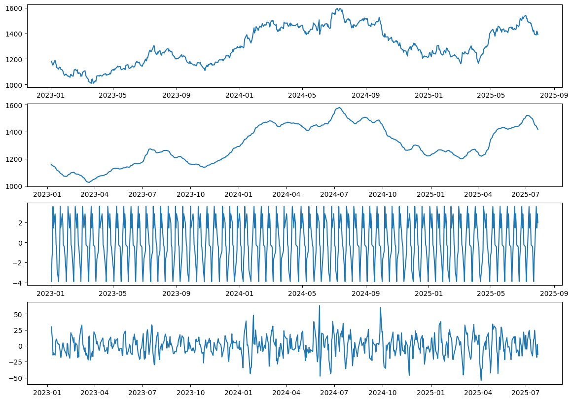
- Assumes fixed seasonal patterns
- Easily influenced by the outliers
- Handle both additive and multiplicative models
- Preferred for multiplicative models
| 0 | |
|---|---|
| Date | |
| 2023-01-02 | 0.0 |
| 2023-01-03 | 0.0 |
| 2023-01-04 | 0.0 |
| 2023-01-05 | 0.0 |
| 2023-01-06 | 0.0 |
| ... | ... |
| 2025-07-25 | 0.0 |
| 2025-07-28 | 0.0 |
| 2025-07-29 | 0.0 |
| 2025-07-30 | 0.0 |
| 2025-07-31 | 0.0 |
637 rows × 1 columns