stationarity – Data Science Lab

A Stationary series is one whose statistical properties such as mean, variance, covariance, and standard deviation do not vary with time, or these stats properties are not a function of time. In other words, stationarity in Time Series also means series without a Trend or Seasonal components.

Constant mean
Constant Variance
Constant covariance

Visual Signs of Non-Stationarity 👀 - Trend: A clear upward or downward movement over time. The mean is not constant.

Seasonality: A pattern that repeats at regular intervals (e.g., yearly, monthly, weekly).
Varying Variance: The spread of the data points increases or decreases over time, making the series appear wider or narrower

Seasonality can be observed in series (d), (h), and (i)
The trend can be observed in series (a), (c), (e), (f), and (i)
Series (b) and (g) are stationary

ADF Test: - Null Hypothesis (HO): Series is non-stationary - Alternate Hypothesis(HA): Series is stationary

Reject the null hypothesis if p-value < 0.05

KPSS Test - Null Hypothesis (HO): Series is trend stationary - Alternate Hypothesis(HA): Series is non-stationary

# Load the libraries
import numpy as np
import pandas as pd
import matplotlib.pyplot as plt

# Using airline passenger dataset (monthly totals)
url = 'https://raw.githubusercontent.com/jbrownlee/Datasets/master/airline-passengers.csv'
df = pd.read_csv(url, parse_dates=['Month'], index_col='Month')
df

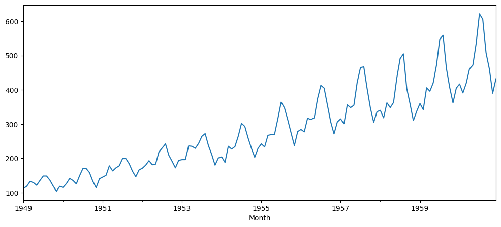
	Passengers
Month
1949-01-01	112
1949-02-01	118
1949-03-01	132
1949-04-01	129
1949-05-01	121
...	...
1960-08-01	606
1960-09-01	508
1960-10-01	461
1960-11-01	390
1960-12-01	432

144 rows × 1 columns

df["Passengers"].plot(figsize = (12,5))

from statsmodels.tsa.stattools import adfuller

dftest = adfuller(df["Passengers"], autolag='AIC')

dfoutput = pd.Series(dftest[0:4], index=['Test Statistic','p-value','#Lags Used','Number of Observations Used'])
for key,value in dftest[4].items():
  dfoutput['Critical Value (%s)'%key] = value
dfoutput

	0
Test Statistic	0.815369
p-value	0.991880
#Lags Used	13.000000
Number of Observations Used	130.000000
Critical Value (1%)	-3.481682
Critical Value (5%)	-2.884042
Critical Value (10%)	-2.578770

dtype: float64

from statsmodels.tsa.stattools import kpss

kpsstest = kpss(df["Passengers"], regression='c', nlags="auto")

/tmp/ipython-input-752976516.py:1: InterpolationWarning: The test statistic is outside of the range of p-values available in the
look-up table. The actual p-value is smaller than the p-value returned.

  kpsstest = kpss(df["Passengers"], regression='c', nlags="auto")

kpss_output = pd.Series(kpsstest[0:3], index=['Test Statistic','p-value','#Lags Used'])
for key,value in kpsstest[3].items():
  kpss_output['Critical Value (%s)'%key] = value
kpss_output

	0
Test Statistic	1.651312
p-value	0.010000
#Lags Used	8.000000
Critical Value (10%)	0.347000
Critical Value (5%)	0.463000
Critical Value (2.5%)	0.574000
Critical Value (1%)	0.739000

dtype: float64

def kpss_test(timeseries):
    print ('Results of KPSS Test:')
    kpss_output = pd.Series(kpsstest[0:3], index=['Test Statistic','p-value','#Lags Used'])
    for key,value in kpsstest[3].items():
        kpss_output['Critical Value (%s)'%key] = value
    print (kpss_output)

The following are the possible outcomes of applying both tests.

Case 1: Both tests conclude that the given series is stationary – The series is stationary
Case 2: Both tests conclude that the given series is non-stationary The series is non-stationary
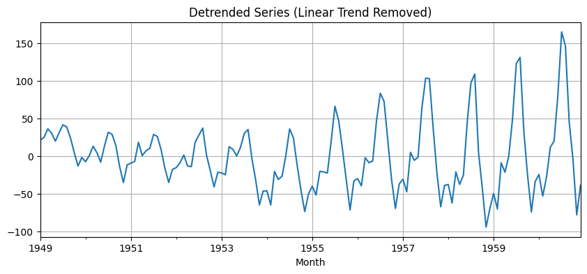
Case 3: ADF concludes non-stationary, and KPSS concludes stationary The series is trend stationary. To make the series strictly stationary, we need to remove the trend in this case. Then we check the detrended series for stationarity.
Case 4: ADF concludes stationary, and KPSS concludes non-stationary The series is difference stationary. Differencing is to be used to make series stationary. Then we check the differenced series for stationarity.

import pandas as pd
import numpy as np
import matplotlib.pyplot as plt
from statsmodels.tsa.stattools import adfuller, kpss
from sklearn.linear_model import LinearRegression


# Plot original series
df['Passengers'].plot(title='Original Airline Passenger Data', figsize=(10, 4))
plt.grid()
plt.show()

# Step 1: Fit linear regression (trend) using sklearn
X = np.arange(len(df)).reshape(-1, 1)       # Time as feature
y = df['Passengers'].values                     # Passenger values
model = LinearRegression().fit(X, y)
trend = model.predict(X)

df['detrended'] = y - model.predict(X)

# Plot detrended series
df['detrended'].plot(title='Detrended Series (Linear Trend Removed)', figsize=(10, 4))
plt.grid()
plt.show()

# Step 2: Stationarity Tests
# ADF Test
adf_orig_p = adfuller(df['Passengers'])[1]
adf_det_p = adfuller(df['detrended'])[1]

# KPSS Test
kpss_orig_p = kpss(df['Passengers'], regression='ct')[1]     # trend + constant
kpss_det_p = kpss(df['detrended'], regression='c')[1]   # constant only

# Step 3: Print Results
print("📊 Stationarity Test Results")
print(f"ADF (Original):     p = {adf_orig_p:.4f} → {'Non-stationary' if adf_orig_p > 0.05 else 'Stationary'}")
print(f"KPSS (Original):    p = {kpss_orig_p:.4f} → {'Non-stationary' if kpss_orig_p < 0.05 else 'Stationary'}")
print(f"ADF (Detrended):    p = {adf_det_p:.4f} → {'Non-stationary' if adf_det_p > 0.05 else 'Stationary'}")
print(f"KPSS (Detrended):   p = {kpss_det_p:.4f} → {'Non-stationary' if kpss_det_p < 0.05 else 'Stationary'}")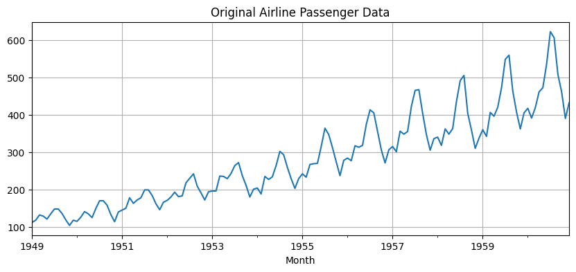

📊 Stationarity Test Results
ADF (Original):     p = 0.9919 → Non-stationary
KPSS (Original):    p = 0.1000 → Stationary
ADF (Detrended):    p = 0.2437 → Non-stationary
KPSS (Detrended):   p = 0.1000 → Stationary

/tmp/ipython-input-2952525283.py:34: InterpolationWarning: The test statistic is outside of the range of p-values available in the
look-up table. The actual p-value is greater than the p-value returned.

  kpss_orig_p = kpss(df['value'], regression='ct')[1]     # trend + constant
/tmp/ipython-input-2952525283.py:35: InterpolationWarning: The test statistic is outside of the range of p-values available in the
look-up table. The actual p-value is greater than the p-value returned.

  kpss_det_p = kpss(df['detrended'], regression='c')[1]   # constant only

Other Links