1. RankConsider the following matrix of size 1000×1000. What is its rank?X=a
1
2
3
⋯
1000
1
2
3
⋯
1000
⋮
1
2
3
⋯
1000
The rank of a matrix is the number of linearly independent columns. Every column of X is some multiple of the first column. X has only one linearly independent column, therefore its rank is 1. This is the mathematical understanding. But what does the rank of a matrix really capture? We will look at it from a different perspective: memory. If the matrix has to be stored in a computer, we need 1000×1000=106 units of memory. Is this the best that we can do? Since all the columns are just multiples of the first column, it is enough if we store the first column along with the multipliers:a
1
⋮
1
,(1,⋯,1000)We need 1000 units of memory to store the first column and 1000 units to store the multipliers. Therefore, we need 2000 units of memory to represent the matrix. Compare the reduction in memory usage: 106/1000≈1000. We have reduced the memory usage by a factor of 1000!Contrast this with another 1000×10000 matrix whose entries are drawn from a standard normal distribution. a
0.12
⋯
1.03
⋮
⋮
-0.09
⋯
-0.1
This is an example of a random matrix. The rank of such a matrix is generally 1000. There doesn't seem to be any simple way to use lesser memory to store such a matrix. We would have to store all the 106 entries. The summary is that matrices that have a low rank offer significant advantages in terms of storage.To put this in terms of the information content, the rank of a matrix can be thought of as a single number that describes the degree of redundant information in the matrix. Lower the rank, greater the redundancy. For example, the first matrix that we saw had rank 1 where the maximum rank could have been 1000. This corresponds to an extreme level of redundancy. Just a handful of the entries in the matrix are absolutely essential and indispensable while the rest can be discarded with impunity. The second example demonstrates the other end of the spectrum where every entry in the matrix is essential for describing the matrix accurately.2. Low-rank ApproximationLet us now look at a simple 3×3 matrix that has full rank:X=a
1.001
2.999
5.001
0.999
3.001
4.999
1.001
2.999
4.999
If we take a closer look, each entry of X is off from an integer by 0.001. If we replace each entry of X by the nearest integer to it, we get:X′=a
1
3
5
1
3
5
1
3
5
The rank of X′ is clearly 1. The difference between X and X′ is at most 0.001 in each cell, so X′ is a very good approximation of X. In fact, X′ is a very good low-rank approximation of X. If we have to store a full rank matrix with a very high level of fidelity, we would have to store every single entry of the matrix in memory. But if we are willing to compromise on this front, then we can store a low-rank approximation of this matrix. As we have argued in the previous section, low-rank matrices bring significant advantages in terms of storage.3. Images as MatricesBut what do matrices have to do with the world of data? Consider the image of a chess board:We could represent a chess board as an 8×8 image. Each cell is a pixel and could either take a value 1 (white) or 0 (black). This is called a grayscale image. Such an image can also be viewed as an 8×8 matrix:C=a
0
1
0
1
0
1
0
1
1
0
1
0
1
0
1
0
0
1
0
1
0
1
0
1
1
0
1
0
1
0
1
0
0
1
0
1
0
1
0
1
1
0
1
0
1
0
1
0
0
1
0
1
0
1
0
1
1
0
1
0
1
0
1
0
What is the rank of this matrix? We immediately see that it has to be 2. Visually, what does this mean? We have a portion of the image that keeps repeating. In the image of the chessboard, it could be either the first two rows or the first two columns. There is a lot of redundancy in the image and this is captured by the rank of the matrix. 4. Image CompressionSuch redundancy is not uncommon in natural images that we see around us:The two columns highlighted in white have been overlaid on the image. Notice how similar these two columns are. But for a few pixels here and there, the two columns are nearly linearly dependent. This suggests that we could look for an approximation of the image that has a lower rank which only captures the most essential and indispensable elements in the original. Such a low-rank approximation would be useful because it would help us reduce the memory consumption with some (minimum) loss of information. Low-rank approximation is one way of compressing an image.5. SVDSVD is one tool that can help us achieve this low-rank approximation. Let us frame the problem in a more mathematically precise manner. Given a m×n matrix A, we wish to find a matrix A′ of rank k, such that the "difference" between them is as small as possible. Here 1⩽k⩽r, where r is the rank of A.
min
rank(A′)=k||A-A′||2The notion of the difference is captured by a matrix norm. Recall that for two vectors x and y, their closeness is measured by the Euclidean norm given by ||x-y||2. The matrix norm is an extension of this idea to matrices. The closer the approximation, smaller the norm. SVD gives us an algorithm to compute this approximation. We will only state a particular way of expressing the singular value decomposition that is relevant to to the problem we wish to solve:
Every real m×n matrix A of rank r can be expressed in the following form:
A=r∑i=1𝜎i⋅ui⋅vTi
𝜎1⩾⋯⩾𝜎r>0 are called the singular values of A. ui∈Rm is called a left singular vector while vj∈Rn is called a right singular vector. Each component of this sum is a unit-rank matrix.
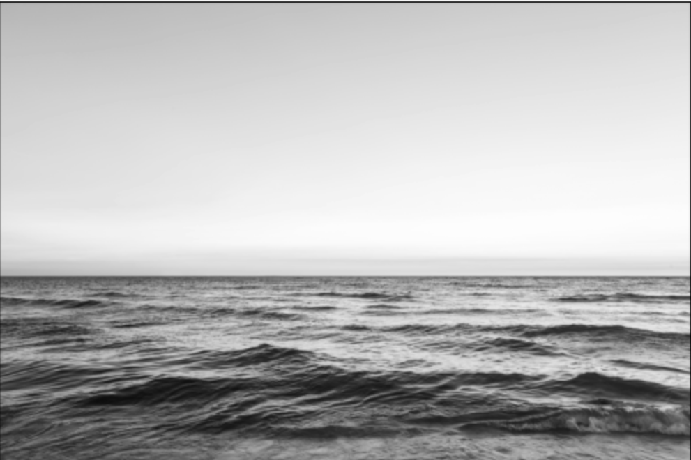
The "best rank-k approximation" of A can then be written down as:A′=k∑i=1𝜎i⋅ui⋅vTiThat is, we keep the first k terms of the sum and discard the rest. Recall that ui⋅vTj is an outer product. It is a matrix of size m×n.6. SVD in ActionLet us see how SVD can help us compress the following image:
To keep things simple, we will work with the grayscale (black-white) version of this image:
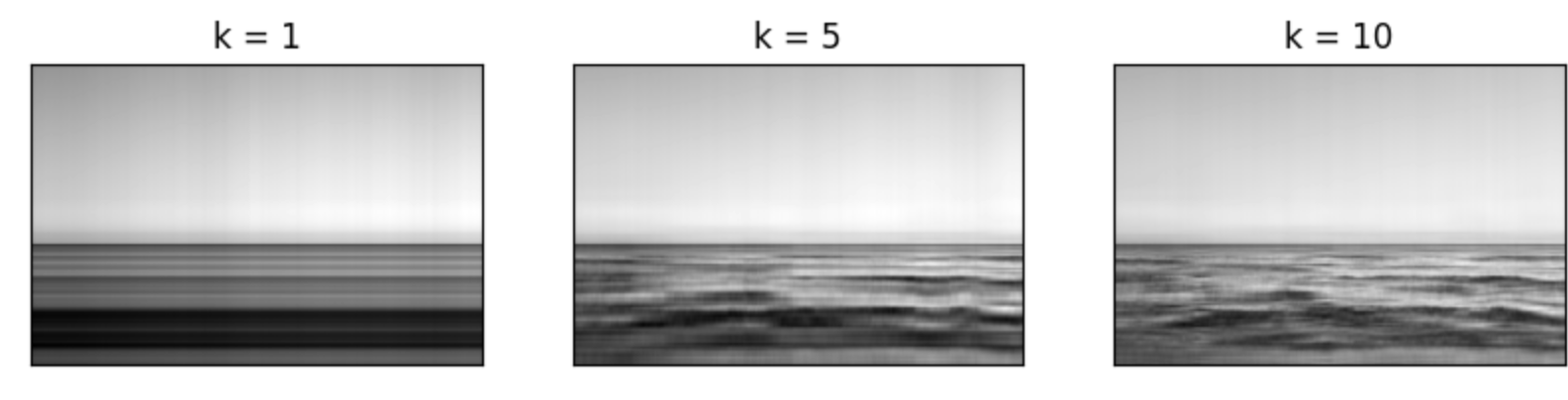
This image is of size 3840×5760. There are 22118400 pixels and it requires about 22 million units of storage! If each pixel is stored as an integer (1 byte), the size of the image on the disk would be roughly 21 MB! Let us see what SVD does to this image. The following plot is the k-rank approximation for five different value of k:
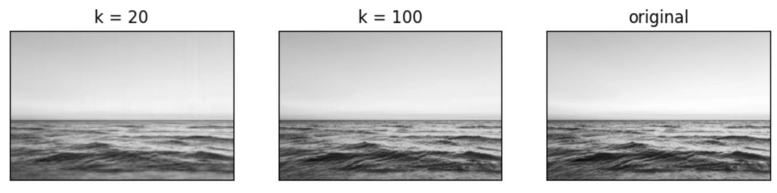
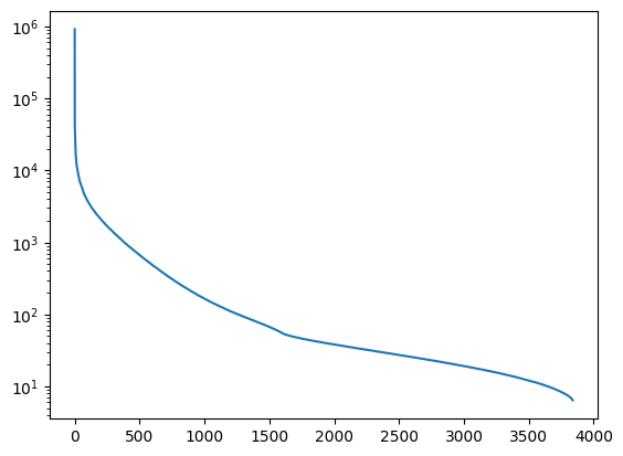
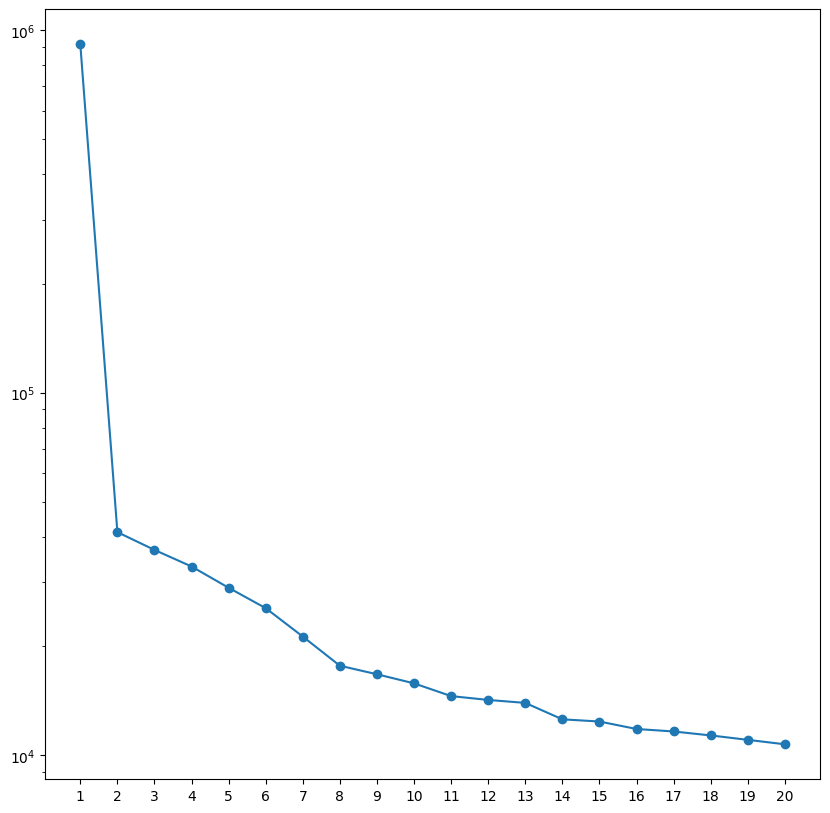
For k=1, we only see a bunch of horizontal lines. This corresponds to a unit rank matrix. Because of the kind of image we have chosen, even a rank-1 approximation seems to capture the most important details of this scene: sea and sky. The rank-5 approximation adds a few more details to the sea, the waves, but it is still blurred. The rank-10 approximation is nearly there. For k=20, the approximation seems almost indistinguishable from the original image.Let us see the amount of compression we are able to achieve if we decide to go with the rank-20 approximation. The approximate image can be represented as:A′=20∑i=1𝜎i⋅ui⋅vTiComputing the image A′ and storing it would not give us any advantage, as we would be back to storing a matrix of size 3840×5760. We can instead just store the 20 singular values and their corresponding singular vectors. To be more precise, we can store the approximate image in this form on our disk:• 20 left singular vectors, each of size 3840• 20 right singular vectors, each of size 5760• 20 singular values, each of size 1 (scalars)This gives us a memory requirement of:20×3840+20×5760+20×1=192020The only catch here is that we would have to store each of these as float values. Let us say each float value occupies 4 bytes of memory. Then, we would require around 192020×4 bytes or 0.75 MB. If we were to store the original image as it is on the disk, we would require 21 MB as computed earlier. We have thus achieved a compression ratio of 21/0.75=28 with the help of SVD's low-rank approximation. In other words, we have reduced the storage cost of the image by a factor of 28!Let us now get a sense of what the singular values look like. The matrix A (image) in our example has size 3840×5760 and it turns out that its rank is 3840. So, there are 3840 singular values for A. The following is a plot of the singular values versus the index, where the singular value axis is in log-scale.
Notice that the largest singular values are somewhere near 106. If we zoom in, we get the following plot for the first 20 singular values:
The first (most important) singular value is nearly two orders of magnitude higher than the rest. The first term in the sum carries the bulk of the information contained in the image. Indeed, one way to view the k-rank approximation is to think about contributions from each unit-rank matrix as being weighted by the singular value. Thus, in the term 𝜎i⋅ui⋅vTi, the singular value 𝜎i controls the importance of this term in the entire sum. The first 20 singular values in this case contain nearly all the essential details in the original image and we can safely discard the rest.7. NotesThis is by no means the only use of SVD or the only way to motivate the topic.• One application of SVD is related to the least squares solution to the linear regression problem that we studied earlier. The SVD of a matrix helps us to compute what is called a pseudo-inverse which helps us in solving the following system of equations -(XTX)w=XTy - even when XTX is not invertible.• PCA can itself been seen as performing SVD on a centered data matrix. More on this in a separate post soon.• Another way of understanding SVD is to treat it as a matrix factorization method: break a matrix into the product of three special matrices, U,𝛴,V, where U and V are orthogonal matrices and 𝛴 is a diagonal-ish matrix.