Plotting Simple Curves
Import and Settings
We will import NumPy and matplotlib. In addition, we will also start with some customised layout for the plot.
Partitioning the real line
In order to plot a curve, we need a set of \(x\) values and the corresponding \(y\) values. Since \(x\) is the independent variable, we need to first generate a list of values for \(x\). This is done using the linspace method in NumPy. np.linspace(a, b, n) generates a sequence of \(n\) numbers that are equally spaced between \(a\) and \(b\), end-points included. As an example:
Here, np.linspace(0, 1, 11) generates a sequence of eleven numbers, starting from \(0\) and ending at \(11\), with equal spacing. We could have also arrived at this result using the arange method by specifying a step size of \(0.1\) and end-point that is greater than \(1\). But clearly, linspace is easier since it avoids these calculations:
Curves
We shall plot several curves, starting from simple curves to more complex ones. In this process, we will also learn how to annotate plots.
Curve-1
Plot \(y = x\) for \(x \in [0, 1]\). Sample \(10\) equally spaced points in this interval, inclusive of endpoints.
In NumPy:
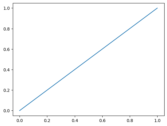
np.plot connects the points that we have specified with the help of a straight line. If we also wish to visualise the location of the individual points, we can add a scatter plot along with the line plot. We will study scatter plots in greater detail in an upcoming notebook.
x = np.linspace(0, 1, 10)
y = x
plt.scatter(x, y)
plt.plot(x, y);
# ; suppresses output, compare with previous cell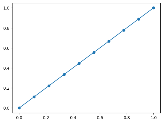
The ; after the plot command suppresses the output. We could have arrived at this line with the help of just two points, since it takes two distinct points to uniquely specify a line:
x = np.array([0, 1])
y = x
# order of plot and scatter doesn't matter here
plt.plot(x, y)
plt.scatter(x, y);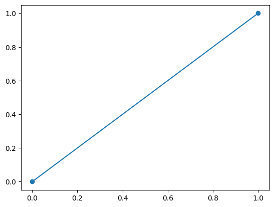
The number of points chosen on the x-axis didn’t matter here. But we will soon see the effect that it has when we plot non-linear functions of the input.
Curve-2
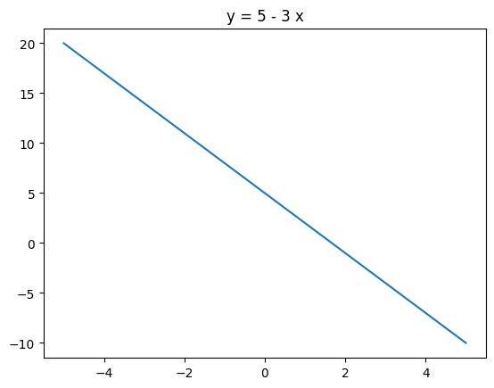
Plot \(y = 5 - 3x\) for \(x \in [-5, 5]\). Sample \(20\) equally spaced points in this interval, inclusive of endpoints. Add a title to the plot which has the equation of the curve.
Curve-3
Plot \(y = x^2\) for \(x \in [-1, 1]\). Try out four different partitions for x:
- \(5\) equally spaced points in this interval, endpoints inclusive
- \(10\) equally spaced points in this interval, endpoints inclusive
- \(20\) equally spaced points in this interval, endpoints inclusive
- \(50\) equally spaced points in this interval, endpoints inclusive
Observe the differences in these four plots. Which one would you choose? Add the equation of the curve as the title of the plot. Also add the x and y-axis to the plot.
# 5 points
x = np.linspace(-1, 1, 5)
y = x ** 2
plt.plot(x, y)
plt.axhline(color='black',
            linestyle='--',
            linewidth=0.8)
plt.axvline(color='black',
            linestyle='--',
            linewidth = 0.8);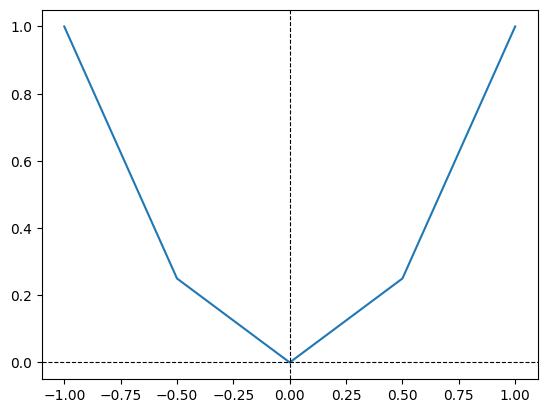
Notice the effect of using a small number of points. Recall that plot.plot connects the points we have given using a straight line. To get a smoother curve that resembles \(y = x^2\), we need a finer partition of the x-axis.
# 50 points
x = np.linspace(-1, 1, 50)
y = x ** 2
plt.plot(x, y)
plt.axhline(color='black',
            linestyle='--',
            linewidth=0.8)
plt.axvline(color='black',
            linestyle='--',
            linewidth = 0.8);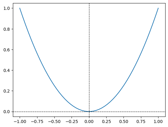
Though the curve appears smooth to our eyes given our finite resolution, note that plt.plot continues to connect consecutive points with a straight lines.
Curve-4
Plot \(y = 3\) and \(x = 5\) on the same plot. Color the first one blue and the second one red. Limit your plot to the region \(x \in [0, 6]\) and \(y \in [0, 6]\).
- Label the x and the y axes.
- Add a suitable title.
- Add a legend.
# y = 3
x = np.array([0, 6])
y = np.array([3, 3])
plt.plot(x, y,
         color='blue',
         label='y = 3')

# x = 5
x = np.array([5, 5])
y = np.array([0, 6])
plt.plot(x, y,
         color='red',
         label='x = 5')

plt.legend()
plt.title('x = 5 and y = 3')
plt.axhline(color='black',
            linestyle='--',
            linewidth=0.8)
plt.axvline(color='black',
            linestyle='--',
            linewidth=0.8);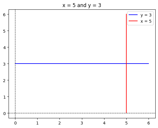
Subplots
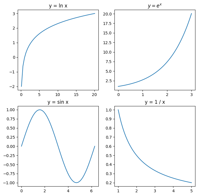
Sometimes we may have to plot multiple curves, each in a separate plot. Plot the following curves, each in a separe plot:
\(y = \ln x, \quad x \in \left( \cfrac{1}{e^2}, e^3 \right)\)
\(y = e^x, \quad x \in (0, 3)\)
\(y = \sin x, \quad x \in [0, 2 \pi]\)
\(y = \cfrac{1}{x}, \quad x \in (1, 5)\)
Title each curve appropriately.
We will first increase the size of the plotting space. This can be manipulated by a parameter called figure.figsize which can be accessed via an object called rcParams, which can be used to change the configuration parameters for various aspects of the plot.
plt.subplot(r, c, ind) divides the plotting region into \(r \times c\) individual plotting windows and selects the plot at index ind. The index is set to \(1\) for the top-left plot and increases by one point from left to right and top to bottom. The top-left plot window has index \(1\), the last window in the first row has index \(c\), and so on.
# Plot-1
plt.subplot(2, 2, 1)
x = np.linspace(1 / np.e ** 2, np.e ** 3)
y = np.log(x)
plt.plot(x, y)
plt.title('y = ln x')

# Plot-2
plt.subplot(2, 2, 2)
x = np.linspace(0, 3)
y = np.exp(x)
plt.plot(x, y)
# $ ... $ is used to render LaTeX
plt.title('$y = e^x$')

# Plot-3
plt.subplot(2, 2, 3)
x = np.linspace(0, 2 * np.pi)
y = np.sin(x)
plt.plot(x, y)
plt.title('y = sin x')

# Plot-4
plt.subplot(2, 2, 4)
x = np.linspace(1, 5)
y = 1 / x
plt.plot(x, y)
plt.title('y = 1 / x');