NumPy Arrays

We will study NumPy arrays in more detail.

import numpy as np

Arrays and Types

It should have become amply clear by now that both vectors and matrices are NumPy arrays. Each array in NumPy has a dimension. Vectors are one-dimensional arrays while matrices are two-dimensional arrays. For example:

\[ \mathbf{x} = \begin{bmatrix} 1\\ 2\\ 3 \end{bmatrix}, \mathbf{M} = \begin{bmatrix} 1 & 2\\ 3 & 4\\ 5 & 6 \end{bmatrix} \]

In NumPy:

x = np.array([1, 2, 3])
print(x.ndim)
M = np.array([
    [1, 2],
    [3, 4],
    [5, 6]
])
print(M.ndim)

1
2

So far we have not looked at the data-types of the elements of an array. Each array in NumPy has a specific type and all the elements of the array partake of this type. Thus we could also characterize a NumPy array as a homogenous collection of elements arranged in a contiguous block in the memory. We shall look at four common types that arrays come in:

• integer
• float
• Boolean
• string

There are variations in some of these types. We won’t go into too much detail here. The type of the NumPy array is stored in the attribute dtype.

An example of int and float types.

x_int = np.array([1, 2, 3])
x_int.dtype

dtype('int64')

x_float = np.array([1.0, 2.0, 3.0])
x_float.dtype

dtype('float64')

A Boolean array is an array of Boolean values. That is, each component is either a True or False. For example:

x_bool = np.array([True, False, True])
x_bool.dtype

dtype('bool')

x_str = np.array(['Red', 'Green', 'Blue'])
x_str.dtype

dtype('<U5')

Sometimes it might be necessary to convert from one data-type to another. We can use astype for this conversion:

x = np.array([1, 2, 3])
y = x.astype(np.float32)
x.dtype, y.dtype

(dtype('int64'), dtype('float32'))

Reshaping

Arrays can be reshaped. We will do a number of examples here.

Example-1: Vector to matrix

We start with a vector:

\[ \mathbf{x} = \begin{bmatrix} 1 & 2 & 3 & 4 & 5 & 6 \end{bmatrix} \]

We can reshape it into the following matrix:

\[ \mathbf{M} = \begin{bmatrix} 1 & 2\\ 3 & 4\\ 5 & 6 \end{bmatrix} \]

In NumPy:

x = np.arange(1, 7)
x

array([1, 2, 3, 4, 5, 6])

M = x.reshape(3, 2)
M

array([[1, 2],
       [3, 4],
       [5, 6]])

Note that we could have packed the six elements into a matrix in two ways:

\[ \begin{bmatrix} 1 & 2\\ 3 & 4\\ 5 & 6 \end{bmatrix}, \quad \quad \begin{bmatrix} 1 & 4\\ 2 & 5\\ 3 & 6 \end{bmatrix} \]

• The one on the left is called row-major ordering or C ordering, where we fill the first row completely, then move on to the second row and so on.
• The one on the right follows a column major ordering or Fortran ordering, where the first column is filled first, followed by the second and so on.

By default, the reshape method follows the row-major ordering. To force a column-major ordering, we can pass an additional argument called order. By default, NumPy follows row-major ordering.

x = np.arange(1, 7)
# F refers to Fortran
M = x.reshape(3, 2,
              order='F')
M

array([[1, 4],
       [2, 5],
       [3, 6]])

Example-2: Matrix to vector

We now start with a matrix:

\[ \mathbf{M} = \begin{bmatrix} 1 & 2 & 3\\ 4 & 5 & 6 \end{bmatrix} \]

We can now reshape it into a vector:

\[ \mathbf{x} = \begin{bmatrix} 1 & 2 & 3 & 4 & 5 & 6 \end{bmatrix} \]

In NumPy:

M = np.array([
    [1, 2, 3],
    [4, 5, 6]
])
M

array([[1, 2, 3],
       [4, 5, 6]])

x = M.reshape(6)
x

array([1, 2, 3, 4, 5, 6])

Alternatively, we could also use the ravel method to achieve this:

M = np.array([
    [1, 2, 3],
    [4, 5, 6]
])
x = M.ravel()
x

array([1, 2, 3, 4, 5, 6])

Note that ravel also follows a row-major ordering by default. To force a column-major ordering, we set order='F':

M = np.array([
    [1, 2, 3],
    [4, 5, 6]
])
x = M.ravel(order='F')
x

array([1, 4, 2, 5, 3, 6])

Example-3: Matrix to matrix

We can reshape a matrix into another matrix as well. Sometimes, we may be lazy to compute both the dimensions. In such cases, we can leave out one of the two dimensions and let NumPy figure it out. The way to do it is to replace the unknown dimension with \(-1\). For example:

\[ \mathbf{M} = \begin{bmatrix} 1 & 2 & 3\\ 4 & 5 & 6 \end{bmatrix} \]

Let us say we want to reshape it in such a way that there are three rows:

\[ \mathbf{P} = \begin{bmatrix} 1 & 2\\ 3 & 4\\ 5 & 6 \end{bmatrix} \]

In NumPy:

M = np.array([
    [1, 2, 3],
    [4, 5, 6]
])
P = M.reshape(3, -1)
P

array([[1, 2],
       [3, 4],
       [5, 6]])

The \(-1\) trick may seem pointless in this case. But it does come in handy when reshaping arrays with several dimensions. In fact, stepping back a bit and looking at the previous example, we can convert a matrix into a vector in the following manner as well:

M = np.array([
    [1, 2, 3],
    [4, 5, 6]
])
x = M.reshape(-1)
x

array([1, 2, 3, 4, 5, 6])

Matrix-vector addition

Sometimes we would have to add a vector to each row or column of a matrix. There are two cases to consider. If the vector to be added is a:

• row vector
• column vector

Row-vector

Consider the following matrix \(\mathbf{M}\) and vector \(\mathbf{b}\):

\[ \mathbf{M} = \begin{bmatrix} 1 & 2 & 3\\ 4 & 5 & 6 \end{bmatrix}, \mathbf{b} = \begin{bmatrix} 1 & 2 & 3 \end{bmatrix} \]

There is a slight abuse of notation as we can’t add a matrix and a vector together. However, the context often makes this clear:

\[ \mathbf{M} + \mathbf{b} = \begin{bmatrix} 2 & 4 & 6\\ 5 & 7 & 9 \end{bmatrix} \]

In NumPy:

M = np.array([
    [1, 2, 3],
    [4, 5, 6]
])
b = np.array([1, 2, 3])
M + b

array([[2, 4, 6],
       [5, 7, 9]])

What does NumPy do here? When presented with an operation that has two arrays (operands) of different shapes, NumPy does an operation called broadcasting. In this case, the shapes of the two operands are \((4, 3)\) and \((3, )\).

Conceptually, the effect of broadcasting is to stretch the second array along the first axis (the rows), creating four copies of the same array so that the two original arrays can be added. In reality, NumPy has a more sophisticated, memory-efficient way of achieving this without actually having to create four copies.

image.png

There are broadcasting rules that specify when two arrays can be combined in an operation. Since this is an introduction to NumPy, we won’t go into great detail. But in the event that we get a broadcasting error, note that we are trying to combine two arrays in an operation that are not compatible for broadcasting.

Column-vector

Now, consider another pair:

\[ \mathbf{M} = \begin{bmatrix} 1 & 2 & 3\\ 4 & 5 & 6 \end{bmatrix}, \mathbf{b} = \begin{bmatrix} 1\\ 2 \end{bmatrix} \]

In this case, we have:

\[ \mathbf{M} + \mathbf{b} = \begin{bmatrix} 2 & 3 & 4\\ 6 & 7 & 8 \end{bmatrix} \]

Let us first try to replicate the same process that we followed while adding a row vector.

try:
    M = np.array([
        [1, 2, 3],
        [4, 5, 6]
    ])
    b = np.array([1, 2])
    M + b
except:
    print('incompatible shapes for broadcasting')

incompatible shapes for broadcasting

This is an instance where the shapes of the arrays are \((2, 3)\) and \((2, )\), which are not compatible for broadcasting according to NumPy’s rules. To make them compatible, what we do is to add an extra dimension to the vector so as to turn it into a column vector.

M = np.array([
    [1, 2, 3],
    [4, 5, 6]
])
b = np.array([1, 2]).reshape(2, 1)
M + b

array([[2, 3, 4],
       [6, 7, 8]])

Advanced Indexing

NumPy has some advanced indexing features that are useful in various applications.

Indexing using arrays

Lists or NumPy arrays themselves can be used as indices to retreive different parts of the array. For example:

\[ \mathbf{x} = \begin{bmatrix} -1 & 0 & 4 & 3 & 7 & 8 & 1 & 9 \end{bmatrix} \]

Let us say that we are interested in retreiving indices: [1, 3, 6].

In NumPy:

# using a NumPy array
x = np.array([-1, 0, 4, 3, 7, 8, 1, 9])
x[np.array([1, 3, 6])]

array([0, 3, 1])

# using a list
x = np.array([-1, 0, 4, 3, 7, 8, 1, 9])
x[[1, 3, 6]]

array([0, 3, 1])

We could also use a Boolean array to index into NumPy arrays.

# using a Boolean array
ind = np.array([False, True, False, True, False, False, True, False])
x = np.array([-1, 0, 4, 3, 7, 8, 1, 9])
x[ind]

array([0, 3, 1])

Filtering particular values

Sometimes we are interested in those elements of the array that possess a particular property:

\[ \mathbf{x} = \begin{bmatrix} 3 & 1 & 5 & -4 & -2 & 1 & 5 \end{bmatrix} \]

Let us try to extract all elements that are positive.

In NumPy:

x = np.array([3, 1, 5, -4, -2, 1, 5])
x > 0

array([ True,  True,  True, False, False,  True,  True])

The operation x > 0 returns a Boolean array which can then be used as an advanced index. Rather than doing this in two steps, we can combine it into a single operation.

x = np.array([3, 1, 5, -4, -2, 1, 5])
x[x > 0]

array([3, 1, 5, 1, 5])

We could also specify multiple conditions using the operators AND, OR and NOT. In NumPy, these three operators are invoked using the following symbols:

• NOT: ~
• AND: &
• OR: |

For example, let us say we want to extract all positive even numbers from the following array:

x = np.array([3, 2, -4, 0, 6, 8, -2])
x[(x > 0) & (x % 2 == 0)]

array([2, 6, 8])

Now onsider two arrays of the same size. We might want to extract all values in the array x for which the corresponding array y satisfies some property. For example, we might want to extract all values of x for which the corresponding y values are either “red” or “green”. More concretely, we can think of y as the array of class labels and x as the array of features in a classification problem.

x = np.array([1, 3, 0, 4, 5, 7, 8])
y = np.array(["red", "green", "yellow", "red", "yellow", "green", "yellow"])
x[(y == "red") | (y == "green")]

array([1, 3, 4, 7])

Alternatively, since y has only three unique strings, we could use the NOT operator:

x = np.array([1, 3, 0, 4, 5, 7, 8])
y = np.array(["red", "green", "yellow", "red", "yellow", "green", "yellow"])
x[~(y == "yellow")]

array([1, 3, 4, 7])

Filtering and follow-up

Sometimes we might want to filter some elements and do some post processing on the resulting array. This is best explained with an example. Consider the ReLU function.

\[ \text{ReLU}(x) = \begin{cases} x, & x \geqslant 0\\ 0, & x < 0 \end{cases} \]

Here, we filter all elements that are non-negative and retain their values while relegating the negative elements to the value zero. This can be achieved using the where method in NumPy:

def relu(x):
    return np.where(x >= 0, x, 0)
relu(np.array([1, -2, 1, 3, -4, -3]))

array([1, 0, 1, 3, 0, 0])

View and Copy

Consider the following operation:

x = np.arange(1, 6)
y = x[:3]
y[0] = 10
x

array([10,  2,  3,  4,  5])

y is a slice of x, the first three elements. However, when the first element of y is modified, the fiirst element of x also undergoes the same modification. This suggests that y is closely tied to x in some way. In NumPy, y is called a view of x.

When creating a view of a NumPy array, the underlying data in the memory is not duplicated. Rather, NumPy figures out a clever way to access the same data using a different object, which we call the view. Slicing always creates views and hence we must be very careful when working with sliced arrays. One more example:

M = np.arange(12).reshape(3, 4)
M

array([[ 0,  1,  2,  3],
       [ 4,  5,  6,  7],
       [ 8,  9, 10, 11]])

N = M[1:3]
N

array([[ 4,  5,  6,  7],
       [ 8,  9, 10, 11]])

N[0] = [3, 2, 1, 0]
M

array([[ 0,  1,  2,  3],
       [ 3,  2,  1,  0],
       [ 8,  9, 10, 11]])

This is rather detailed example. Note that N is initialized as the slice of the matrix M, the last two rows of M, to be precise. N is a view. In the next cell, the first row of N is modified in-place. Since N is a view, this ends up changing the underlying data which is shared with M as well. The first row of N corresponds to the second row of M .

In some situations, we might want to create a copy of the data such that the two objects do not share the underlying data. This is done using the copy method:

M = np.arange(12).reshape(3, 4)
N = M[1:3].copy()
N[0] = [3, 2, 1, 0]
M

array([[ 0,  1,  2,  3],
       [ 4,  5,  6,  7],
       [ 8,  9, 10, 11]])

Notice that M is undisturbed by the changes to M.

Some operations produce views while others produce copies. We noted that simple slicing always returns views. On the other hand, advanced indexing always returns copies. For example:

x = np.array([1, -1, 4, 5, -2, -3, 8])
y = x[x > 0]
y

array([1, 4, 5, 8])

Let’s change y in-place and see what happens:

y[:3] = [1, 1, 1]
x

array([ 1, -1,  4,  5, -2, -3,  8])

x remains undisturbed since y is a copy and not a view. To determine if an object is a view or copy of another object, we can use the following command:

y.base is None

True

If y is a copy, then the y.base will be None. However, if y is a view, then it will point to the parent object. For example:

x = np.array([1, 2, 3, 4])
y = x[:2]
y.base

array([1, 2, 3, 4])

Before we end this section, it is important to know that the reshape method returns a view whenever possible. As an example:

x = np.arange(10)
M = x.reshape(5, 2)
M.base is None

False

Notice that M is a view here and not a copy.

Operations along axes

Sometimes we may wish to do some operations on all the row-vectors of a matrix or all the column-vectors of the matrix. The idea of axis is important to understand how these operations can be done.

Top-bottom

Top-bottom operations are done on row-vectors. For example, consider the matrix:

\[ \mathbf{A} = \begin{bmatrix} 1 & 2 & 3 & 4\\ 5 & 6 & 7 & 8 \end{bmatrix} \]

The sum of the row-vectors of the matrix is a vector:

\[ \text{rsum}(\mathbf{A}) = \begin{bmatrix} 6 & 8 & 10 & 12 \end{bmatrix} \]

In NumPy:

A = np.arange(1, 9).reshape(2, 4)
A.sum(axis=0)

array([ 6,  8, 10, 12])

Left-right

Left-right operations are done on column-vectors.

\[ \mathbf{A} = \begin{bmatrix} 1 & 2 & 3 & 4\\ 5 & 6 & 7 & 8 \end{bmatrix} \]

The sum of the column-vectors of the matrix is a vector:

\[ \text{csum}(\mathbf{A}) = \begin{bmatrix} 10\\ 26 \end{bmatrix} \]

In NumPy:

A.sum(axis=1)

array([10, 26])

Sum, Mean, Variance, Norm

Let us look at a few more important operations that sweep accross a particular axis of an array. We shall use the following matrix to demonstrate this:

\[ \mathbf{M} = \begin{bmatrix} 1 & 2 & 3\\ 4 & 5 & 6\\ 7 & 8 & 9 \end{bmatrix} \]

Let us find the following quantities:

• sum of column-vectors
• mean of row-vectors
• variance of column-vectors

M = np.arange(1, 10).reshape(3, 3)
M

array([[1, 2, 3],
       [4, 5, 6],
       [7, 8, 9]])

# sum of column vectors
M.sum(axis=1)

array([ 6, 15, 24])

# mean of row vectors
M.mean(axis=0)

array([4., 5., 6.])

# variance of column vectors
M.var(axis=1)

array([0.66666667, 0.66666667, 0.66666667])

Stacking arrays

Sometimes, we would need to stack arrays. Consider the two matrices:

\[ \mathbf{A} = \begin{bmatrix} 1 & 2\\ 3 & 4 \end{bmatrix}, \mathbf{B} = \begin{bmatrix} 5 & 6\\ 7 & 8 \end{bmatrix} \]

There are two ways to stack these two matrices:

• top-bottom
• left-right

Top-bottom

We could stack the two matrices along the rows, \(\mathbf{A}\) on top of \(\mathbf{B}\):

\[ \mathbf{C} = \begin{bmatrix} 1 & 2\\ 3 & 4\\ 5 & 6\\ 7 & 8 \end{bmatrix} \]

In NumPy:

A = np.array([
    [1, 2],
    [3, 4]
])
B = np.array([
    [5, 6],
    [7, 8]
])
np.concatenate((A, B),
               axis=0)

array([[1, 2],
       [3, 4],
       [5, 6],
       [7, 8]])

Left-right

We could stack the two matrices along the columns, \(\mathbf{A}\) to the left of \(\mathbf{B}\):

\[ \mathbf{C} = \begin{bmatrix} 1 & 2 & 5 & 6\\ 3 & 4 & 7 & 8\\ \end{bmatrix} \]

In NumPy:

A = np.array([
    [1, 2],
    [3, 4]
])
B = np.array([
    [5, 6],
    [7, 8]
])
np.concatenate((A, B),
               axis=1)

array([[1, 2, 5, 6],
       [3, 4, 7, 8]])

Misc functions

Let us look at a few other functions that are quite useful:

• unique
• maximum
• max and argmax
• min and argmin
• sort and argsort

x = np.array([10, -3, 2, 15, 5, -3, 2, 12])
x

array([10, -3,  2, 15,  5, -3,  2, 12])

np.unique(x)

array([-3,  2,  5, 10, 12, 15])

# max, argmax
np.max(x), np.argmax(x)

(np.int64(15), np.int64(3))

# min, argmin
np.min(x), np.argmin(x)

(np.int64(-3), np.int64(1))

# sort, argsort
np.sort(x), np.argsort(x)

(array([-3, -3,  2,  2,  5, 10, 12, 15]), array([1, 5, 6, 2, 4, 0, 7, 3]))

These functions also work on arrays of dimension more than one. If we specify an axis, the maximum will be computed along that axis.

M = np.array([
    [1, 3, 5],
    [3, -1, -4]
])
np.max(M, axis = 1)

array([5, 3])

A similar mechanism holds for sort:

M = np.array([
    [1, 3, 5],
    [3, -1, -4],
    [5, -4, 10]
])
np.sort(M, axis = 0)

array([[ 1, -4, -4],
       [ 3, -1,  5],
       [ 5,  3, 10]])

Comparing Arrays

To check if two arrays are equal element-wise, we use np.array_equal:

x = np.array([1, 2, 3])
y = np.array([1, 2, 3])
np.array_equal(x, y)

True

x = np.array([1, 2, 4])
y = np.array([1, 2, 3])
np.array_equal(x, y)

False

Just using x == y would result in a Boolean array. This can’t be used in an if-statement. If we insist on using it, the result is an exception:

try:
    x = np.array([1, 2, 4])
    y = np.array([1, 2, 3])
    if x == y:
        print('works')
except:
    print('does not work')

does not work

Sometimes the arrays being compared may not be exactly equal because of finite precision used to represent real numbers. In such situation, we can use np.allclose and specify the tolerance we want.

x = np.array([1.001, 2.001, 3.001])
y = np.array([1, 2, 3])
np.allclose(x, y,
            rtol=0,
            atol=1e-2)

True

np.allclose(x, y, atol=delta, rtol=0) will return true if the absolute value of the difference between every pair of corresponding elements of x and y is at most delta. That is, the following condition should evaluate to True for all indices:

abs(x[i] - y[i]) <= delta

Higher dimensional Arrays

So far we have studied 1D and 2D NumPy arrays. We also have higher dimensional arrays. A classic example of a 3D NumPy array is an image dataset. Let us take a look at the legendary MNIST dataset.

import matplotlib.pyplot as plt
from keras.datasets import mnist

train, test = mnist.load_data()

X, y = train

print(X.shape)
print(y.shape)

(60000, 28, 28)
(60000,)

We see that X is a 3D array. The first dimension is the index of the sample, the other two correspond to the location of the pixels in an image.

Let us look at a sample image. It is of shape \(28 \times 28\).

# extract an image with label "7"
img = X[y == 7][0]
print(img.shape)
# Plot this image
plt.imshow(img, cmap = 'gray');

(28, 28)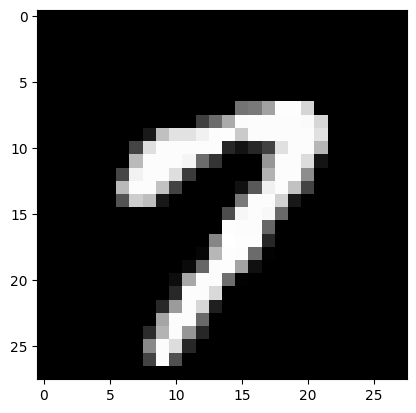

If we wish to treat \(X\) this as a tabular dataset, we can would have to reshapt it so that it is of the form \(d \times n\). Here is where the index \(-1\) comes in handy:

print('Original shape', X.shape)
X_reshaped = X.reshape(60000, -1).T
print('Final shape', X_reshaped.shape)

Original shape (60000, 28, 28)
Final shape (784, 60000)

We can now treat this as a data-matrix of shape \(d \times n\), where \(d = 784\) and \(n = 60,000\). Notice that we didn’t have to compute the value \(784\) explicitly and left NumPy to do that task for us. Let us quickly check whether X_reshaped is a view or a copy.

X_reshaped.base is X

True

It turns out that X_reshaped is a view.