Week 3: K-means

Colab Link: Click here!

Construction of a dataset with implicit clustering

import matplotlib.pyplot as plt
import numpy as np

plt.rcParams['figure.dpi'] = 150

N = 200
np.random.seed(42)

c1 = np.random.randn(N//3, 2) + np.array([8, 8])
c2 = np.random.randn(N//3, 2) + np.array([8, -1])
c3 = np.random.randn(N//3, 2) + np.array([-1, -1])

X = np.concatenate((c1, c2, c3))
plt.scatter(X[:, 0], X[:, 1], s=10);
plt.axis('equal')
plt.show()

Is PCA Enough?

# Perform PCA on X

plt.figure(figsize=(12, 5))

X_mean = X.mean(axis=0)

X_centered = X - X_mean
cov_X = np.cov(X_centered.T)
eig_val, eig_vec = np.linalg.eigh(cov_X)
pc_vec = eig_vec[:,-1] / eig_vec[:,-1][0]
x_range = np.array([-7, 8])

plt.subplot(1, 2, 1)
plt.scatter(X[:, 0], X[:, 1], s=10);
plt.axis('equal')
plt.plot(x_range + X_mean[0], x_range * pc_vec[1] + X_mean[1], color='black')

plt.subplot(1, 2, 2)
plt.scatter(X[:, 0], X[:, 1], s=10);
X_proj = np.array([i * eig_vec[:, -1] + X_mean for i in X_centered @ eig_vec[:, -1]])
plt.scatter(X_proj[:, 0], X_proj[:, 1], s=20, color='red');
plt.axis('equal')
plt.plot(x_range + X_mean[0], x_range * pc_vec[1] + X_mean[1], color='black')

plt.show()

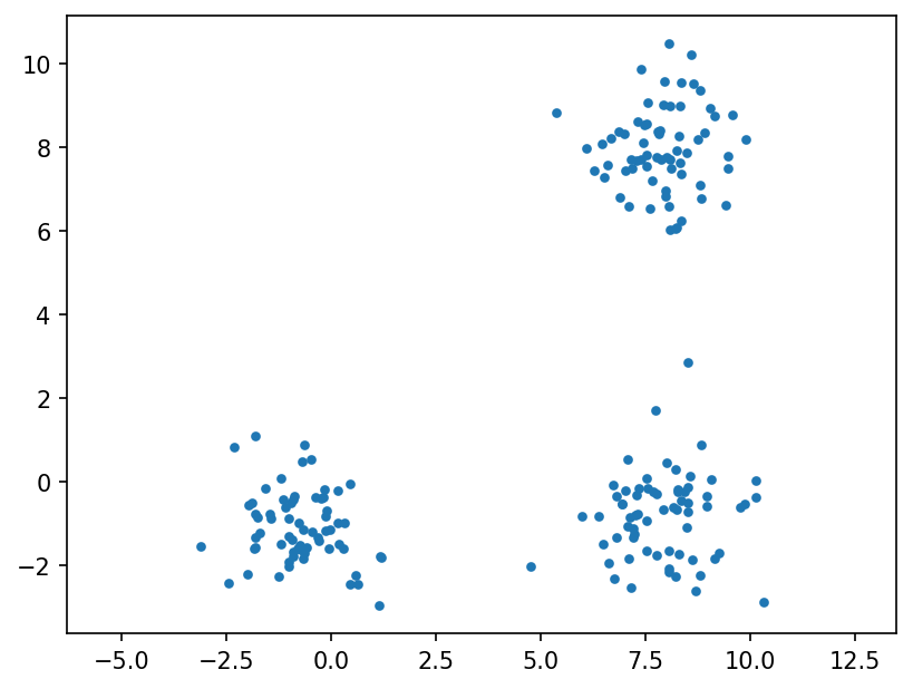
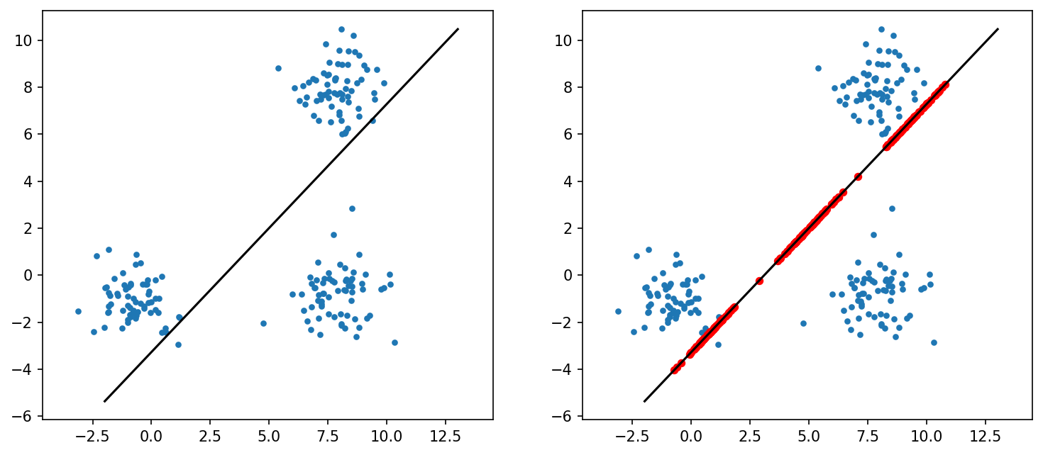
We notice the dataset generated above has some implicit “clustering”. When we run PCA however, no information about this phenomenon is captured in the representations generated by it. Hence, a different problem formulation is required, which is able to capture this similarity in datasets that we postulate to follow this pattern.

K-means Clustering - Lloyd’s Algorithm

• It is an unsupervised learning algorithm
• The algorithm tries to capture “similarity” between datapoints, and assign a cluster indicator for each clique.

Problem Definition

In this context, the objective becomes the following:

\underset{z \in S}{\text{min }} \sum_{i=1}^{n}||x_i - μ_{z_i}||^2_2

Where: - x_i denotes the i’th datapoint - z_i denotes the cluster indicator of x_i - μ_{z_i} denotes the mean of the cluster with indicator z_i - S denotes the set of all possible cluster assignments. Note that S is finite

def obj(X, cluster_centers):
  return sum([np.min([np.linalg.norm(x_i - cluster_center)**2 for cluster_center in cluster_centers]) for x_i in X])

Algorithm Strategy

1. Initialization Step : Assign random datapoints from the dataset as the cluster centers
2. Cluster Assignment Step : For every datapoint x_i, assign a cluster indicator z_i = \underset{j \in [1, 2, ..., n]}{\text{min }} ||x_i - μ_j||^2_2
3. Recompute cluster centers : For every cluster indicator j \in [1, 2, ..., n] recompute μ_j = \frac{\sum_{i=1}^{n}x_i \cdot \mathbf{1}(z_i=j)}{\sum_{i=1}^{n} \mathbf{1}(z_i=j)}
4. Repeat steps 2 and 3 until convergence.

Convergence in accordance to the objective is established, since the following can be shown: - The set of all possible cluster assignments S is finite. - The objective function value strictly decreases after every iteration of Lloyd’s.

The initialization for K-Means can be done in smarter ways than a random initialization - which improve the chance of lloyd’s converging to a good cluster assignment; with a lesser number of iterations.

It is important to note that the final assignment need not necessarily be the best answer (global optima) to the objective function, but it is good enough in practice.

Initialization Step

n points from the dataset are randomly chosen as cluster centers, where n is the number of clusters - a hyperparameter

n = 3
# cluster_centers = X[np.random.choice(len(X), 3)]
cluster_centers = X[[70, 85, 80]]

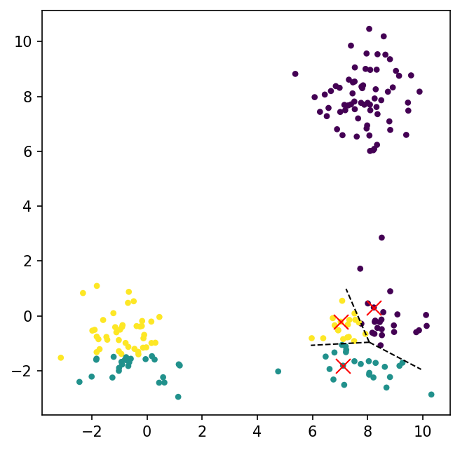
Cluster Assignment Step

For every datapoint, the cluster indicator whose center is closest to the datapoint is assigned as its cluster.

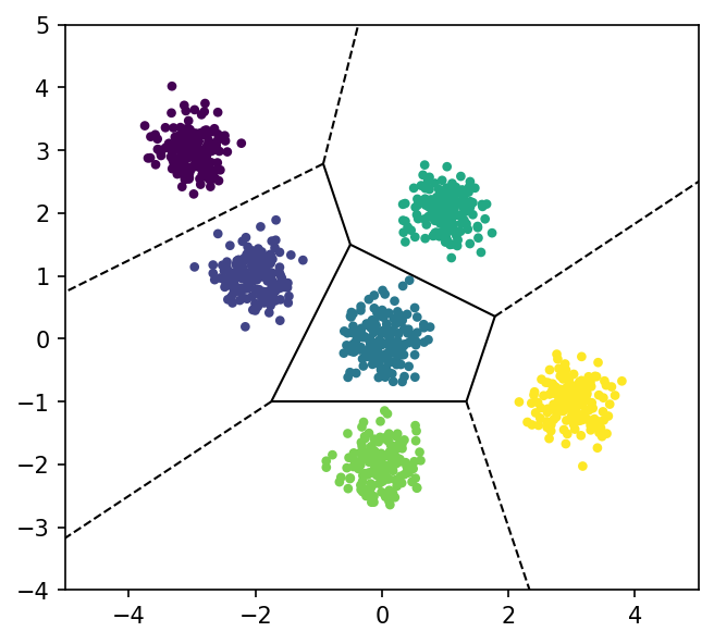
from scipy.spatial import Voronoi, voronoi_plot_2d

def cluster_assignment(X, cluster_centers):
  z = np.zeros(X.shape[0])
  for i in range(X.shape[0]):
    z[i] = np.argmin([np.linalg.norm(X[i] - cluster_center) for cluster_center in cluster_centers])
  return z

z = cluster_assignment(X, cluster_centers)

fig, (ax) = plt.subplots(1, 1)
fig.set_size_inches(5, 5)

ax.scatter(X[:, 0], X[:, 1], c=z, s=10);
ax.scatter(cluster_centers[:, 0], cluster_centers[:, 1], marker = 'x', s = 100, color = 'red', linewidth=1)

vor = Voronoi(cluster_centers)
voronoi_plot_2d(vor, ax=ax, show_points=False, show_vertices=False);

ax.axis('equal');

For every cluster, there is a corresponding interesction of half-spaces - called Voronoi regions. The K-Means algorithm, equivalently, is trying to find the most optimal Voronoi partition of the space, that minimizes the objective function.

Recompute Means/Cluster Centers

For every cluster, the cluster center is updated to the mean of the points in the cluster.

def recompute_clusters(X, z):
  cluster_centers = np.array([np.mean(X[z == i], axis = 0) for i in range(n)])
  return cluster_centers

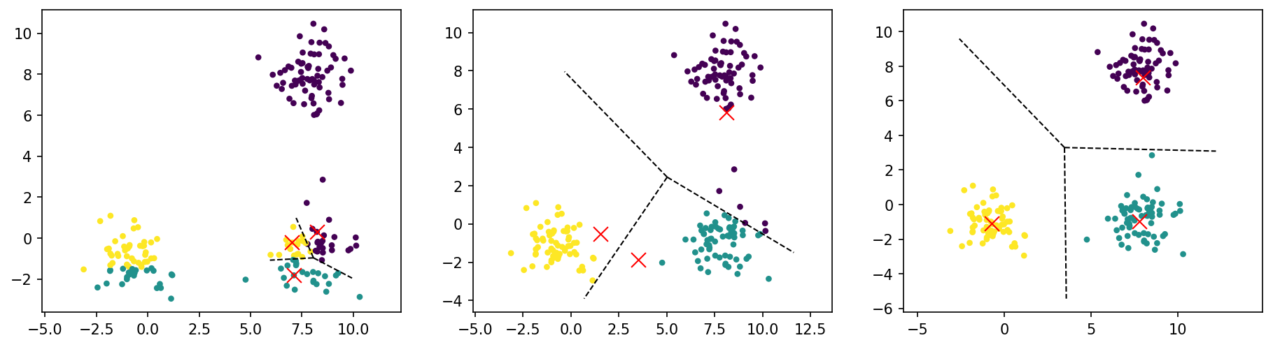
Iteration of K-means

• Assign clusters based on new cluster centers.
• Recompute cluster centers based on new clusters.

fig, ax = plt.subplots(1, 3)
fig.set_size_inches(15, 3.75)

for i in range(3):

  z = cluster_assignment(X, cluster_centers) # cluster_centers -> NEW cluster assignment ->

  ax[i].scatter(X[:, 0], X[:, 1], c=z, s=10);
  ax[i].scatter(cluster_centers[:, 0], cluster_centers[:, 1], marker = 'x', s = 100, color = 'red', linewidth=1)
  vor = Voronoi(cluster_centers)
  voronoi_plot_2d(vor, ax=ax[i], show_points=False, show_vertices=False)
  ax[i].axis('equal');

  cluster_centers = recompute_clusters(X, z) # -> cluster assignment -> NEW cluster centers

Generate a complex dataset with 6 clusters

We make use of the convienient make_blobs data generator from the scikit-learn ibrary.

import matplotlib.pyplot as plt
import numpy as np
from sklearn.datasets import make_blobs

cen = [(-3, 3), (-2, 1), (0, 0), (1, 2), (0, -2), (3, -1)]
X, ideal_z = make_blobs(n_samples=1000, centers=cen, n_features=2, cluster_std=0.3, random_state=13, center_box=(-3, 3))

fig, ax = plt.subplots()
ax.scatter(X[:, 0], X[:, 1], s=10, c=ideal_z)
vor = Voronoi(cen)
voronoi_plot_2d(vor, ax=ax, show_points=False, show_vertices=False);
fig.set_size_inches(5, 4.5)
ax.axis([-5, 5, -4, 5])

(-5.0, 5.0, -4.0, 5.0)

# the make_blobs generator returns the optimal/good cluster assignment along with the dataset
# this function checks whether the result from lloyd's is equivalent to the optimal assignment

def ideal_check(ideal, obtained):
  mapping = dict([(i, -1) for i in range(n)])

  for i in range(len(ideal)):
    if mapping[ideal[i]] == -1:
      mapping[ideal[i]] = obtained[i]
    elif mapping[ideal[i]] != obtained[i]:
      return False

  return True

Lloyd’s Algorithm Definition

from IPython.display import HTML
from matplotlib import animation

def lloyds(cluster_centers, X, z, artists = [], animate=True, fig=None, ax=None, ax1=None, n_iter=0, n = len(cen)):
  loss = []
  if fig is None and animate:
    fig, (ax, ax1) = plt.subplots(1, 2, figsize=(10, 4.15))
    title = ax.set_title('')
    artists = []

  if animate:
      frame = []
      frame.append(ax.scatter(X[:, 0], X[:, 1], c=z, s=10))
      frame.append(ax.scatter(cluster_centers[:, 0], cluster_centers[:, 1], marker = 'x', s = 100, color = 'red', linewidth=1))
      frame.append(ax.text(0.5, 1.05, f'Iteration {n_iter} | Cluster Assignment', transform=ax.transAxes, ha="center"))

      vor = Voronoi(cluster_centers)
      d = voronoi_plot_2d(vor, ax=ax, show_points=False, show_vertices=False);
      frame += list(d.axes[0].lines[-1:] + d.axes[0].collections[-2:])
      ax.axis([-5, 5, -4, 5])

      loss.append(obj(X, cluster_centers))
      m = 1
      frame.append(ax1.scatter([0], [loss[0]], color='red', marker='x', s=30))
      frame.append(ax1.text(0.5, 1.05, 'Objective Function', transform=ax1.transAxes, ha="center"))
      frame.append(ax1.text(0.5, -0.1, 'Iterations', transform=ax1.transAxes, ha="center"))

      artists.append(frame)

  converged = False
  while not converged:

    # cluster_centers = recompute_clusters(X, z)
    for i in range(n):
      cluster_points = X[z==i]
      if len(cluster_points)>0:
        cluster_centers[i] = np.mean(cluster_points, axis=0)

    n_iter += 1

    # Modified cluster assignment step
    converged = True

    if animate:
      frame = []
      frame.append(ax.scatter(X[:, 0], X[:, 1], c=z, s=10))
      frame.append(ax.scatter(cluster_centers[:, 0], cluster_centers[:, 1], marker = 'x', s = 100, color = 'red', linewidth=1))
      frame.append(ax.text(0.5, 1.05, f'Iteration {n_iter} | Cluster Recomputation', transform=ax.transAxes, ha="center"))

      vor = Voronoi(cluster_centers)
      d = voronoi_plot_2d(vor, ax=ax, show_points=False, show_vertices=False);
      frame += list(d.axes[0].lines[-1:] + d.axes[0].collections[-2:])
      ax.axis([-5, 5, -4, 5])

      for i in range(0, len(loss)-1, 2):
        frame.append(list(ax1.plot([i/2, (i+2)/2], [loss[i], loss[i+1]], color='red', marker='x', markersize=5))[0])

      loss.append(obj(X, cluster_centers))
      frame.append(list(ax1.plot([(len(loss)-2)/2, (len(loss)-1)/2], [loss[-2], loss[-1]], color='red', linestyle=':'))[0])
      # lines = list(ax1.plot(np.arange(len(loss))/2, loss, color='red', marker='xo', markersize=6))
      # frame += lines
      frame.append(ax1.text(0.5, 1.05, 'Objective Function', transform=ax1.transAxes, ha="center"))
      frame.append(ax1.text(0.5, -0.1, 'Iterations', transform=ax1.transAxes, ha="center"))

      artists.append(frame)

    for i in range(len(X)):
      z_i = np.argmin([np.linalg.norm(X[i] - cluster_center) for cluster_center in cluster_centers])

      if z_i != z[i]:
        z[i] = z_i
        converged = False

    if animate and not converged:
      frame = []
      frame.append(ax.scatter(X[:, 0], X[:, 1], c=z, s=10))
      frame.append(ax.scatter(cluster_centers[:, 0], cluster_centers[:, 1], marker = 'x', s = 100, color = 'red', linewidth=1))
      frame.append(ax.text(0.5, 1.05, f'Iteration {n_iter} | Cluster Re-assignment', transform=ax.transAxes, ha="center"))

      vor = Voronoi(cluster_centers)
      d = voronoi_plot_2d(vor, ax=ax, show_points=False, show_vertices=False);
      frame += list(d.axes[0].lines[-1:] + d.axes[0].collections[-2:])
      ax.axis([-5, 5, -4, 5])

      loss.append(obj(X, cluster_centers))
      m = 1
      for i in range(0, len(loss)-1, 2):
        frame.append(list(ax1.plot([i/2, (i+2)/2], [loss[i], loss[i+1]], color='red', marker='x', markersize=5))[0])

      frame.append(ax1.text(0.5, 1.05, 'Objective Function', transform=ax1.transAxes, ha="center"))
      frame.append(ax1.text(0.5, -0.1, 'Iterations', transform=ax1.transAxes, ha="center"))

      artists.append(frame)

  if animate:
    plt.close()
    return fig, (ax, ax1), cluster_centers, artists
  else:
    return cluster_centers, n_iter

Random Initialization

We now run Lloyd’s algorithm on the dataset with random initialization. We use the ideal_check function to see whether the obtained cluster from lloyd’s is optimal; else we re-run it again.

An animation using Matplotlib’s ArtistAnimation is shown to illustrate the working of this strategy.

cluster_centers = X[np.random.choice(len(X), n)]
z = cluster_assignment(X, cluster_centers)

fig, ax, final_clusters, artists = lloyds(cluster_centers, X, z)

while not ideal_check(cluster_assignment(X, final_clusters), ideal_z):

  cluster_centers = X[np.random.choice(len(X), n)]
  z = cluster_assignment(X, cluster_centers)
  fig, ax, final_clusters, artists = lloyds(cluster_centers, X, z)

anim = animation.ArtistAnimation(fig, artists, interval=500, repeat=False, blit=False);
HTML(anim.to_jshtml())

Once Loop Reflect

Some initializations do not give a good clustering

cluster_centers = X[np.random.choice(len(X), n)]
z = cluster_assignment(X, cluster_centers)
fig, ax, final_clusters, artists = lloyds(cluster_centers, X, z)

while ideal_check(cluster_assignment(X, final_clusters), ideal_z):
  cluster_centers = X[np.random.choice(len(X), n)]
  z = cluster_assignment(X, cluster_centers)
  fig, ax, final_clusters, artists = lloyds(cluster_centers, X, z)

anim = animation.ArtistAnimation(fig, artists, interval=500, repeat=False, blit=False);
HTML(anim.to_jshtml())

Once Loop Reflect

Smart Initialization | k-means++

k-means++ is an intitialization step which tries to improve the chance for Lloyd’s algorithm to converge to a good clustering.

The exact algorithm is as follows:

• Choose one center uniformly at random among the data points.
• For each data point x not chosen yet, compute D(x)^2, the squared distance between x and the nearest center that has already been chosen.
• Choose one new data point at random as a new center, using a weighted probability distribution where a point x is chosen with probability proportional to D(x)^2.
• Repeat Steps 2 and 3 until k centers have been chosen.

After choosing k cluster centers, we proceed as usual with Lloyd’s algorithm.

The intuition behind this approach is that spreading out the k initial cluster centers is a good thing: the first cluster center is chosen uniformly at random from the data points that are being clustered, after which each subsequent cluster center is chosen from the remaining data points with probability proportional to its squared distance from the point’s closest existing cluster center.

def plusplus(animate=True, n = len(cen)):
  initial_clusters = np.array(X[np.random.choice(len(X), 1)])

  if animate:
      artists = []
      fig, (ax, ax1) = plt.subplots(1, 2, figsize=(10, 4.15), dpi=150)

      a = ax.scatter(X[:, 0], X[:, 1], color="pink", s=10);
      b = ax.scatter(initial_clusters[:, 0], initial_clusters[:, 1], marker = 'x', s = 200, color = 'red', linewidth=1);
      c = ax.text(0.5, 1.05, f'K-Means ++', transform=ax.transAxes, ha="center")

      artists.append([a, c])

      c = ax.text(0.5, 1.05, f'K-Means ++ | Initialization 1', transform=ax.transAxes, ha="center")
      artists.append([a, b, c])

  for i in range(1, n):
    # Rescore based on selected clusters
    scores = np.array([min([np.linalg.norm(datapoint-cluster)**2 for cluster in initial_clusters]) for datapoint in X])

    # Normalize scores to probability
    probabilities = scores/scores.sum()

    initial_clusters = np.append(initial_clusters, X[np.random.choice(len(X), 1, p=probabilities)], axis=0)
    if animate:
      a = ax.scatter(X[:, 0], X[:, 1], color="pink", s=10);
      b = ax.scatter(initial_clusters[:, 0], initial_clusters[:, 1], marker = 'x', s = 200, color = 'red', linewidth=1);
      c = ax.text(0.5, 1.05, f'K-Means ++ | Initialization {i+1}', transform=ax.transAxes, ha="center")

      artists.append([a, b, c])

  if animate:
    return fig, (ax, ax1), initial_clusters, artists

  return initial_clusters

We now run Lloyd’s with K-means++ initialization strategy. The plusplus function does this smart intialization for us; and is configured to plot frames for each point’s initialization, which we use to visualize in our animation.

# cluster_centers = X[np.random.choice(len(X), n)]
fig, (ax, ax1), cluster_centers, artists = plusplus()
z = cluster_assignment(X, cluster_centers)
fig, (ax, ax1), final_clusters, artists = lloyds(cluster_centers, X, z, artists=artists, fig=fig, ax=ax, ax1=ax1)

while not ideal_check(cluster_assignment(X, final_clusters), ideal_z):
  fig, ax, cluster_centers, artists = plusplus()
  z = cluster_assignment(X, cluster_centers)
  fig, (ax, ax1), final_clusters, artists = lloyds(cluster_centers, X, z, artists=artists, fig=fig, ax=ax, ax1=ax1)

anim = animation.ArtistAnimation(fig, artists, interval=500, repeat=False, blit=False);
HTML(anim.to_jshtml())

Once Loop Reflect

Choice of K - Elbow Method

K = list(range(1, 16))
obj_vals = []
for k in K:
  obj_vals_k = []
  for _ in range(3):
    cluster_centers = plusplus(animate=False, n=k)
    cluster_centers, n_iter = lloyds(cluster_centers, X, cluster_assignment(X, cluster_centers), animate=False, n=k)
    obj_vals_k.append(obj(X, cluster_centers))
  obj_vals.append(min(obj_vals_k))

penalties = [100*i for i in K]

plt.figure(figsize=(12, 4))
plt.subplot(1, 2, 1)
plt.plot(K, obj_vals, label='Obj. Value')
plt.plot(K, penalties, linestyle='--', label='Penalty')
plt.xlabel('Choice of K')
plt.legend()

plt.subplot(1, 2, 2)
plt.plot(K, [penalties[i] + obj_vals[i] for i in range(15)])
plt.xlabel('Choice of K')
plt.ylabel('Objective Function + Penalty(K)');
plt.axvline(x=min(zip(K, [penalties[i] + obj_vals[i] for i in range(15)]), key=lambda i: i[1])[0], color='red', label='Minimum Value')
plt.legend()

<matplotlib.legend.Legend at 0x7c57f3588af0>

Comparison of Initialization Strategies - Random vs. K-Means++

For each initialization strategy, we conduct 1000 experiments and record the following:

• Number of Iterations to converge
• SSE (objective value) for final cluster centers
• Number of convergences that are “ideal” (global optimum)
• Time taken from intialization to convergence

Experiments

Random Initialization

from timeit import default_timer as timer

noof_trials = 1000

random = {'ideals' : 0,
          'SSE' : [],
          'iters' : [],
          'time' : []}

exp_start = timer()
for _ in range(noof_trials):

  start = timer()
  cluster_centers = X[np.random.choice(len(X), n)]
  final_clusters, n_iter = lloyds(cluster_centers, X, cluster_assignment(X, cluster_centers), animate=False)

  random['time'].append(timer()-start)
  random['ideals'] += int(ideal_check(ideal_z, cluster_assignment(X, final_clusters)))
  random['SSE'].append(obj(X, final_clusters))
  random['iters'].append(n_iter)

print(f'Experiment done in {timer()-exp_start:.2f} seconds')

Experiment done in 670.24 seconds

K-Means++ Initialization

kmplusplus = {'ideals' : 0,
              'SSE' : [],
              'iters' : [],
              'time' : []}

exp_start = timer()
for _ in range(noof_trials):

  start = timer()
  cluster_centers = plusplus(animate=False)
  final_clusters, n_iter = lloyds(cluster_centers, X, cluster_assignment(X, cluster_centers), animate=False)

  kmplusplus['time'].append(timer()-start)
  kmplusplus['ideals'] += int(ideal_check(ideal_z, cluster_assignment(X, final_clusters)))
  kmplusplus['SSE'].append(obj(X, final_clusters))
  kmplusplus['iters'].append(n_iter)

print(f'Experiment done in {timer()-exp_start:.2f} seconds')

Experiment done in 539.66 seconds

Results

SSE Comparison

plt.style.use('seaborn-v0_8')

fig = plt.figure(figsize=(12, 5))
fig.suptitle('Initialization Comparison | SSE')

ax1 = plt.subplot(121)
ax1.hist(random['SSE'], bins=30)
ax1.set_title('Random')
ax1.set_ylabel('Frequency')
ax1.set_xlabel('SSE')

ax2 = plt.subplot(122, sharex=ax1, sharey=ax1)
ax2.hist(kmplusplus['SSE'], bins=30)
ax2.set_title('K-Means++')
ax2.set_ylabel('Frequency')
ax2.set_xlabel('SSE')

plt.show()

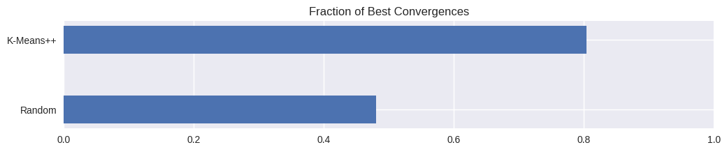
plt.figure(figsize=(12, 2))
plt.title('Fraction of Best Convergences')
plt.barh(['Random', 'K-Means++'], [random['ideals']/noof_trials, kmplusplus['ideals']/noof_trials], height=0.4);
plt.xlim([0, 1]);

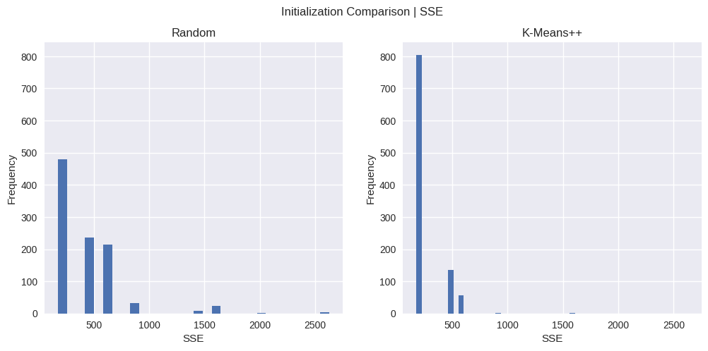
The SSE for the optimal cluster assignment for this particular dataset is around 175. We observe from the above charts that K-Means++ does indeed have a higher chance (0.8) of converging to this as compared to Vanilla K-Means (0.5).

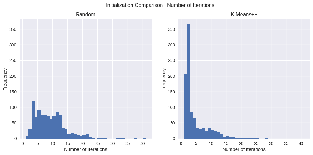
Number of Iterations Comparison

fig = plt.figure(figsize=(12, 5))
fig.suptitle('Initialization Comparison | Number of Iterations')

ax1 = plt.subplot(121)
ax1.hist(random['iters'], bins=max(random['iters'])-min(random['iters']))
ax1.set_title('Random')
ax1.set_ylabel('Frequency')
ax1.set_xlabel('Number of Iterations')

ax2 = plt.subplot(122, sharex=ax1, sharey=ax1)
ax2.hist(kmplusplus['iters'], bins=max(kmplusplus['iters'])-min(kmplusplus['iters']))
ax2.set_title('K-Means++')
ax2.set_ylabel('Frequency')
ax2.set_xlabel('Number of Iterations')

plt.show()

For Vanilla K-Means, we observe that the number of iterations has quite a bit of variation, with an average of 8.75 iterations to convergence.

K-Means++ has a relatively smaller spread, with an average of 4.2 iterations to convergence (post intialization).

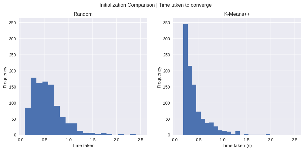
Time Taken Comparison

fig = plt.figure(figsize=(12, 5))
fig.suptitle('Initialization Comparison | Time taken to converge')

ax1 = plt.subplot(121)
ax1.hist(random['time'], bins=20)
ax1.set_title('Random')
ax1.set_ylabel('Frequency')
ax1.set_xlabel('Time taken')

ax2 = plt.subplot(122, sharex=ax1, sharey=ax1)
ax2.hist(kmplusplus['time'], bins=20)
ax2.set_title('K-Means++')
ax2.set_ylabel('Frequency')
ax2.set_xlabel('Time taken (s)')

plt.show()

np.array(kmplusplus['time']).mean()

0.4248704458820016

Similar to the results for number of iterations, the time taken till convergence also has a wide spread for Random Initialization, with an average of 0.55s. K-Means++ has an average of 0.42s.

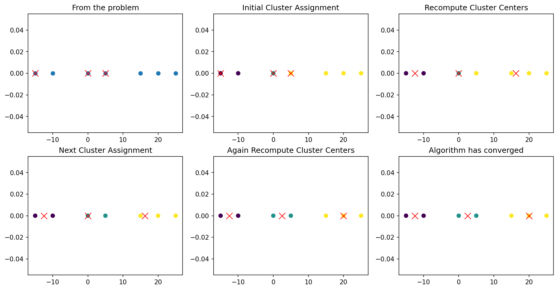
Worked-out Examples

K-Means

K-Means with k = 3 for X = [-15, -10, 0, 5, 15, 20, 25] with mean clusters μ = [-15, 0, 5]

plt.figure(figsize=(15, 7.5))
# From the problem
x = np.expand_dims(np.array([-15, -10, 0, 5, 15, 20, 25]), axis=1)
clusters = np.expand_dims(np.array([-15, 0, 5]), axis=1)
plt.subplot(2, 3, 1)
plt.scatter(x[:,0], np.zeros(x.shape[0]));
plt.scatter(clusters[:, 0], np.zeros(3), marker = 'x', s = 100, color = 'red', linewidth=1);
plt.title('From the problem')

# Initial Cluster Assignment
z = cluster_assignment(x, clusters)
plt.subplot(2, 3, 2)
plt.scatter(x[:,0], np.zeros(x.shape[0]), c=z);
plt.scatter(clusters[:, 0], np.zeros(3), marker = 'x', s = 100, color = 'red', linewidth=1);
plt.title('Initial Cluster Assignment')

# Recompute Cluster Centers
clusters = recompute_clusters(x, z)
plt.subplot(2, 3, 3)
plt.scatter(x[:,0], np.zeros(x.shape[0]), c=z);
plt.scatter(clusters[:, 0], np.zeros(3), marker = 'x', s = 100, color = 'red', linewidth=1);
plt.title('Recompute Cluster Centers')

# Next Cluster Assignment
z = cluster_assignment(x, clusters)
plt.subplot(2, 3, 4)
plt.scatter(x[:,0], np.zeros(x.shape[0]), c=z);
plt.scatter(clusters[:, 0], np.zeros(3), marker = 'x', s = 100, color = 'red', linewidth=1);
plt.title('Next Cluster Assignment')

# Again Recompute Cluster Centers
clusters = recompute_clusters(x, z)
plt.subplot(2, 3, 5)
plt.scatter(x[:,0], np.zeros(x.shape[0]), c=z);
plt.scatter(clusters[:, 0], np.zeros(3), marker = 'x', s = 100, color = 'red', linewidth=1);
plt.title('Again Recompute Cluster Centers')

# Cluster Assignment - No Change
# Algorithm has converged
z = cluster_assignment(x, clusters)
plt.subplot(2, 3, 6)
plt.scatter(x[:,0], np.zeros(x.shape[0]), c=z);
plt.scatter(clusters[:, 0], np.zeros(3), marker = 'x', s = 100, color = 'red', linewidth=1);
plt.title('Algorithm has converged');

K-Means++

For the dataset below, k-means++ algorithm is run with k=2. Find the probability that \mathbf{x}_2, \mathbf{x}_1 are chosen as the initial clusters, in that order.

\left\{\mathbf{x_{1}} \ =\ \begin{bmatrix} 0\\ 2 \end{bmatrix} ,\mathbf{\ x_{2}} \ =\ \begin{bmatrix} 2\\ 0 \end{bmatrix} ,\ \mathbf{x_{3}} \ =\ \begin{bmatrix} 0\\ 0 \end{bmatrix} ,\ \mathbf{x_{4}} \ =\ \begin{bmatrix} 0\\ -2 \end{bmatrix} ,\ \mathbf{x_{5}} \ =\ \begin{bmatrix} -2\\ 0 \end{bmatrix}\right\}

dataset = np.array([[0, 2], [2, 0], [0, 0], [0, -2], [-2, 0]])
probabilities = np.array([1/len(dataset) for _ in range(len(dataset))])
print('Initial Probablities:', probabilities)
clusters = []
answer = 1

# First we select x2 = [2,0]
clusters.append(dataset[1])
answer *= probabilities[1]

# Rescore based on selected clusters
scores = np.array([min([np.linalg.norm(datapoint-cluster)**2 for cluster in clusters]) for datapoint in dataset])

# Normalize scores to probability
probabilities = scores/scores.sum()
print('Probabilities after selecting x2: ', [round(i, 3) for i in probabilities])

# Now we select x1 = [0,2]
clusters.append(dataset[0])
answer *= probabilities[0]

print('Probability of selecting [x2 x1]:', round(answer, 3))

Initial Probablities: [0.2 0.2 0.2 0.2 0.2]
Probabilities after selecting x2:  [0.222, 0.0, 0.111, 0.222, 0.444]
Probability of selecting [x2 x1]: 0.044