Discriminative Models - Perceptron; Logistic Regression

Note

Feedback/Correction: Click here!.

Perceptron Learning Algorithm

The Perceptron Learning Algorithm (PLA) is a supervised learning algorithm widely employed for binary classification tasks. Its primary objective is to determine a decision boundary that effectively separates the two classes in the dataset. This algorithm belongs to the class of discriminative classification methods as it focuses on modeling the boundary between classes instead of characterizing the underlying probability distribution of each class.

Let \(D=\{(\mathbf{x}_1, y_1), \ldots, (\mathbf{x}_n,y_n)\}\) represent the dataset, where \(\mathbf{x}_i \in \mathbb{R}^d\) and \(y_i \in \{0, 1\}\).

The algorithm is founded on the following assumptions:

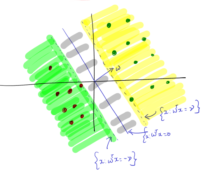
\(P(y=1|\mathbf{x}) = 1\) if \(\mathbf{w}^\mathbf{T}\mathbf{x}\geq0\), otherwise \(P(y=1|\mathbf{x}) = 0\).
Linear Separability Assumption: The Linear Separability Assumption is a fundamental assumption made in various machine learning algorithms, including the Perceptron Learning Algorithm. It posits that the classes to be classified can be accurately separated by a linear decision boundary. In other words, there exists a hyperplane in the feature space that can effectively segregate the data points of the two classes.

The objective function is defined as follows:

\[ \min _{h \in \mathcal{H}} \sum _{i=1} ^n \mathbb{1}\left ( h(\mathbf{x}_i) \neq y_i \right ) \]

Even if \(\mathcal{H}\) accounts only for the Linear Hypotheses, this problem is generally considered NP-Hard.

Under the Linear Separability Assumption, assuming the existence of \(\mathbf{w} \in \mathbb{R}^d\) such that \(\text{sign}(\mathbf{w}^\mathbf{T}\mathbf{x}_i)=y_i\) holds for all \(i \in \{1, 2, \ldots, n\}\), the PLA solves the convergence problem using an iterative algorithm. The algorithm proceeds as follows:

Initialize \(\mathbf{w}^0 = \mathbf{0} \in \mathbb{R}^d\)
Until Convergence:
- Select a \((\mathbf{x}_i, y_i)\) pair from the dataset
- If \(\text{sign}(\mathbf{w}^\mathbf{T}\mathbf{x}_i)==y_i\)
  - Do nothing
- Else
  - Update the weight vector: \(\mathbf{w}^{(t+1)} = \mathbf{w}^t + \mathbf{x}_iy_i\)
- End

Analysis of the Update Rule

For a given training example \((\mathbf{x}, y)\), where \(\mathbf{x}\) represents the input and \(y\) represents the correct output (either \(1\) or \(-1\)), the perceptron algorithm updates the weight vector \(\mathbf{w}\) according to the following rules:

If the perceptron’s prediction on \(\mathbf{x}\) is correct (i.e., \(\text{sign}(\mathbf{w}^\mathbf{T}\mathbf{x}_i)==y_i\)), no update is performed.
If the perceptron’s prediction on \(\mathbf{x}\) is incorrect (i.e., \(\text{sign}(\mathbf{w}^\mathbf{T}\mathbf{x}_i)\neq y_i\)), the weights are updated by adding the product of the input vector and the correct output to the current weight vector: \(\mathbf{w}^{(t+1)} = \mathbf{w}^t + \mathbf{x}_iy_i\).
It is important to note that the update occurs solely in response to the current data point. Consequently, data points that were previously classified correctly may not be classified similarly in future iterations.

This update rule effectively adjusts the decision boundary in the direction of correct classification for the misclassified example. The algorithm is guaranteed to converge to a linearly separable solution if the data is indeed linearly separable. However, if the data is not linearly separable, the perceptron algorithm may not converge to a solution.

Further Assumptions

We introduce three additional assumptions:

Linear Separability with \(\gamma\)-Margin: A dataset \(D=\{(\mathbf{x}_1, y_1), \ldots, (\mathbf{x}_n,y_n)\}\) is considered linearly separable with a \(\gamma\)-margin if there exists \(\mathbf{w}^* \in \mathbb{R}^d\) such that \((\mathbf{w}^{*T}\mathbf{x}_i)y_i\geq\gamma\) holds for all \(i\), where \(\gamma>0\).

Linear Separability with \(\gamma\)-Margin

Radius Assumption: Let \(R>0 \in \mathbb{R}\) be a constant such that \(\forall i \in D\), \(||\mathbf{x}_i||\leq R\). In other words, \(R\) denotes the length of the data point farthest from the center.
Normal Length for \(\mathbf{w}^*\): Assume that \(\mathbf{w}^*\) has unit length.

Proof of Convergence of Perceptron Algorithm

We denote the current mistake number as \(l\). Based on our previous findings, we can observe the following:

\[\begin{align*} \mathbf{w}^{l} &= \mathbf{w}^{l-1} + \mathbf{x}y \\ ||\mathbf{w}^{l}||^2&=||\mathbf{w}^{l-1} + \mathbf{x}y||^2 \\ &=(\mathbf{w}^{l-1} + \mathbf{x}y)^T(\mathbf{w}^{l-1} + \mathbf{x}y) \\ &=||\mathbf{w}^{l-1}||^2 + 2(\mathbf{w}^{{l-1}T}\mathbf{x})y+ ||\mathbf{x}||^2y^2 \\ \therefore ||\mathbf{w}^{l}||^2&\leq ||\mathbf{w}^{l-1}||^2 + R^2 \\ &\leq (||\mathbf{w}^{l-2}||^2 + R^2) + R^2 \\ &\leq ||\mathbf{w}^0||^2 + lR^2 \\ \therefore ||\mathbf{w}^{l}||^2&\leq lR^2 \hspace{6em} \ldots[1] \end{align*}\]

Furthermore, we have:

\[\begin{align*} \mathbf{w}^{l} &= \mathbf{w}^{l-1} + \mathbf{x}y \\ (\mathbf{w}^{l})^T\mathbf{w}^* &= (\mathbf{w}^{l-1} + \mathbf{x}y)^T\mathbf{w}^* \\ &= \mathbf{w}^{{l-1}T}\mathbf{w}^* + (\mathbf{w}^{*T}\mathbf{x})y \\ \therefore (\mathbf{w}^{l})^T\mathbf{w}^* &\geq \mathbf{w}^{{l-1}T}\mathbf{w}^* + \gamma \\ &\geq (\mathbf{w}^{l-2T}\mathbf{w}^* + \gamma) + \gamma \\ &\geq \mathbf{w}^{0T}\mathbf{w}^* + l\gamma \\ \therefore (\mathbf{w}^{l})^T\mathbf{w}^* &\geq l\gamma \\ ((\mathbf{w}^{l})^T\mathbf{w}^*)^2 &\geq l^2\gamma^2 \\ ||\mathbf{w}^{l}||^2||\mathbf{w}^*||^2 &\geq l^2\gamma^2 \hspace{0.5em}\ldots\text{Using the Cauchy-Schwarz inequality}\\ \therefore ||\mathbf{w}^{l}||^2 &\geq l^2\gamma^2 \hspace{6em} \ldots[2] \end{align*}\]

Combining equations \([1]\) and \([2]\), we obtain:

\[\begin{align*} l^2\gamma^2 &\leq ||\mathbf{w}^{l}||^2 \leq lR^2 \\ l^2\gamma^2 &\leq lR^2 \\ \therefore l &\leq \frac{R^2}{\gamma^2} \end{align*}\]

Consequently, the above equation establishes an upper bound on the number of mistakes for datasets conforming to the Linear Separability with \(\gamma\)-Margin property and having a finite radius \(R\). This result demonstrates the convergence of the perceptron algorithm.

Logistic Regression

Sigmoid Function

Until now, we have utilized the \(\text{sign}\) function to determine the class for the output. However, what if we also wish to obtain the probabilities associated with these outputs?

Let \(z=\mathbf{w}^\mathbf{T}\mathbf{x}\), where \(z \in \mathbb{R}\). How can we map \([-\infty, \infty]\rightarrow[0,1]\)? To address this, we introduce the Sigmoid Function, defined as follows:

\[ g(z) = \frac{1}{1+e^{-z}} \]

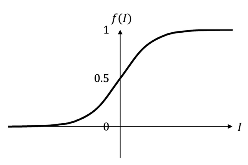
The sigmoid function is commonly employed in machine learning as an activation function for neural networks. It exhibits an S-shaped curve, making it well-suited for modeling processes with a threshold or saturation point, such as logistic growth or binary classification problems.

For large positive input values, the sigmoid function approaches 1, while for large negative input values, it approaches 0. When the input value is 0, the sigmoid function output is exactly 0.5.

The term “sigmoid” is derived from the Greek word “sigmoides,” meaning “shaped like the letter sigma” (\(\Sigma\)). The sigmoid function’s characteristic S-shaped curve resembles the shape of the letter sigma, which likely influenced the function’s name.

Logistic Regression

Logistic regression is a statistical method used to analyze and model the relationship between a binary (two-valued) dependent variable and one or more independent variables. The independent variables can be either continuous or categorical. The main objective of logistic regression is to estimate the probability that the dependent variable belongs to one of the two possible values, given the independent variable values.

In logistic regression, the dependent variable is modeled as a function of the independent variables using a logistic (sigmoid) function. This function generates an S-shaped curve ranging between 0 and 1. By transforming the output of a linear combination of the independent variables using the logistic function, logistic regression provides a probability estimate that can be used for classifying new observations.

Let \(D=\{(\mathbf{x}_1, y_1), \ldots, (\mathbf{x}_n,y_n)\}\) denote the dataset, where \(\mathbf{x}_i \in \mathbb{R}^d\) and \(y_i \in \{0, 1\}\).

We know that:

\[ P(y=1|\mathbf{x}) = g(\mathbf{w}^\mathbf{T}\mathbf{x}_i) = \frac{1}{1+e^{-\mathbf{w}^\mathbf{T}\mathbf{x}}} \]

Using the maximum likelihood approach, we can derive the following expression:

\[\begin{align*} \mathcal{L}(\mathbf{w};\text{Data}) &= \prod _{i=1} ^{n} (g(\mathbf{w}^\mathbf{T}\mathbf{x}_i))^{y_i}(1- g(\mathbf{w}^\mathbf{T}\mathbf{x}_i))^{1-y_i} \\ \log(\mathcal{L}(\mathbf{w};\text{Data})) &= \sum _{i=1} ^{n} y_i\log(g(\mathbf{w}^\mathbf{T}\mathbf{x}_i))+(1-y_i)\log(1- g(\mathbf{w}^\mathbf{T}\mathbf{x}_i)) \\ &= \sum _{i=1} ^{n} y_i\log\left(\frac{1}{1+e^{-\mathbf{w}^\mathbf{T}\mathbf{x}_i}}\right)+(1-y_i)\log\left(\frac{e^{-\mathbf{w}^\mathbf{T}\mathbf{x}_i}}{1+e^{-\mathbf{w}^\mathbf{T}\mathbf{x}_i}}\right) \\ &= \sum _{i=1} ^{n} \left [ (1-y_i)(-\mathbf{w}^\mathbf{T}\mathbf{x}_i) - \log(1+e^{-\mathbf{w}^\mathbf{T}\mathbf{x}_i}) \right ] \end{align*}\]

Therefore, our objective, which involves maximizing the log-likelihood function, can be formulated as follows:

\[ \max _{\mathbf{w}}\sum _{i=1} ^{n} \left [ (1-y_i)(-\mathbf{w}^\mathbf{T}\mathbf{x}_i) - \log(1+e^{-\mathbf{w}^\mathbf{T}\mathbf{x}_i}) \right ] \]

However, a closed-form solution for this problem does not exist. Therefore, we resort to using gradient descent for convergence.

The gradient of the log-likelihood function is computed as follows:

\[\begin{align*} \nabla \log(\mathcal{L}(\mathbf{w};\text{Data})) &= \sum _{i=1} ^{n} \left [ (1-y_i)(-\mathbf{x}_i) - \left( \frac{e^{-\mathbf{w}^\mathbf{T}\mathbf{x}_i}}{1+e^{-\mathbf{w}^\mathbf{T}\mathbf{x}_i}} \right ) (-\mathbf{x}_i) \right ] \\ &= \sum _{i=1} ^{n} \left [ -\mathbf{x}_i + \mathbf{x}_iy_i + \mathbf{x}_i \left( \frac{e^{-\mathbf{w}^\mathbf{T}\mathbf{x}_i}}{1+e^{-\mathbf{w}^\mathbf{T}\mathbf{x}_i}} \right ) \right ] \\ &= \sum _{i=1} ^{n} \left [ \mathbf{x}_iy_i - \mathbf{x}_i \left( \frac{1}{1+e^{-\mathbf{w}^\mathbf{T}\mathbf{x}_i}} \right ) \right ] \\ \nabla \log(\mathcal{L}(\mathbf{w};\text{Data})) &= \sum _{i=1} ^{n} \left [ \mathbf{x}_i \left(y_i - \frac{1}{1+e^{-\mathbf{w}^\mathbf{T}\mathbf{x}_i}} \right ) \right ] \end{align*}\]

Utilizing the gradient descent update rule, we obtain:

\[\begin{align*} \mathbf{w}_{t+1} &= \mathbf{w}_t + \eta_t\nabla \log(\mathcal{L}(\mathbf{w};\text{Data})) \\ &= \mathbf{w}_t + \eta_t \left ( \sum _{i=1} ^{n} \mathbf{x}_i \left(y_i - \frac{1}{1+e^{-\mathbf{w}^\mathbf{T}\mathbf{x}_i}} \right ) \right ) \end{align*}\]

Kernel and Regularized Versions

It is possible to argue that \(\mathbf{w}^*=\displaystyle\sum _{i=1} ^{n}\alpha_i\mathbf{x}_i\), thereby allowing for kernelization. For additional information, please refer to this link.

The regularized version of logistic regression can be expressed as follows:

\[ \min _{\mathbf{w}}\sum _{i=1} ^{n} \left [ \log(1+e^{-\mathbf{w}^\mathbf{T}\mathbf{x}_i}) + \mathbf{w}^\mathbf{T}\mathbf{x}_i(1-y_i) \right ] + \frac{\lambda}{2}||\mathbf{w}||^2 \]

Here, \(\frac{\lambda}{2}||\mathbf{w}||^2\) serves as the regularizer, and \(\lambda\) is determined through cross-validation.