Support Vector Machines
Feedback/Correction: Click here!.
PDF Link: Click here!
Perceptron and Margin Maximization in Linear Separability
In this week, we explore the concept of perceptron learning in the context of linearly separable datasets with a specified margin, denoted as \(\gamma\). The dataset is defined as \(D=\{(\mathbf{x_1}, y_1), \ldots, (\mathbf{x_n},y_n)\}\), where \(\mathbf{x_i} \in \mathbb{R}^d\) represents data points and \(y_i \in \{-1, 1\}\) indicates their respective classes.
Defining Key Parameters
We begin by introducing essential parameters:
Weight Vector: Let \(\mathbf{w^*} \in \mathbb{R}^d\) be the weight vector such that \((\mathbf{w^{*T}x_i})y_i\ge\gamma\) for all \(i\). This weight vector ensures the desired margin \(\gamma\).
Bounding Radius: We define \(R>0 \in \mathbb{R}\) such that for all \(i\), \(||\mathbf{x_i}||\le R\). This represents a constraint on the norm of input data.
With these parameters established, we can formulate the upper bound on the number of mistakes made by the perceptron learning algorithm: \[ \text{\#mistakes} \le \frac{R^2}{\gamma^2} \]
Observations and Objectives
Observations
We make several observations regarding the perceptron learning algorithm:
- The “quality” of the solution depends on the margin \(\gamma\).
- The number of mistakes is influenced by the margin associated with \(\mathbf{w^*}\).
- The weight vector \(\mathbf{w_{perc}}\) need not be identical to \(\mathbf{w^*}\).
Goal: Margin Maximization
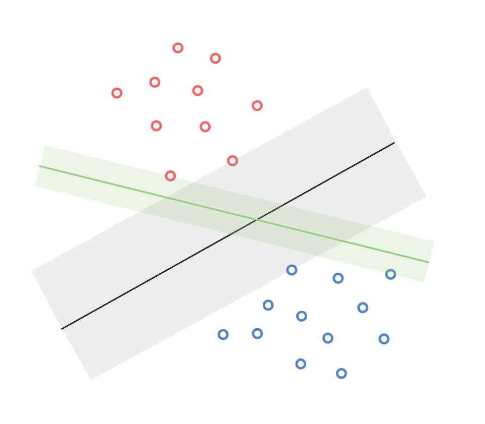
Given these observations, our overarching goal is to find the solution that maximizes the margin. It is crucial to note that a single dataset can have multiple linear classifiers with varying margins, as depicted in the diagram below:
To formalize our objective, we aim to maximize the margin \(\gamma\): \[ \max_{\mathbf{w},\gamma} \gamma \]
Subject to the following constraints: \[\begin{align*} (\mathbf{w^T x_i})y_i &\ge \gamma \quad \text{for all } i \\ ||\mathbf{w}||^2 &= 1 \end{align*}\]
Reformulating the Objective
To simplify our objective, we can express \(\gamma\) in terms of the width of \(\mathbf{w}\): \[ \max_{\mathbf{w}} \text{width}(\mathbf{w}) \]
Subject to the constraint: \[ (\mathbf{w^T x_i})y_i \ge 1 \quad \text{for all } i \]
Width Calculation
The width of the margin, denoted as \(\text{width}(\mathbf{w})\), can be calculated as the distance between two parallel margins. Consider two points \(\mathbf{x}\) and \(\mathbf{z}\) lying on opposite sides of the decision boundary such that \(\mathbf{w^T x}=-1\) and \(\mathbf{w^T z}=1\) or vice versa.
Let \(\mathbf{x_1}\) and \(\mathbf{x_2}\) be two points on the margins and opposite sides of the decision boundary.
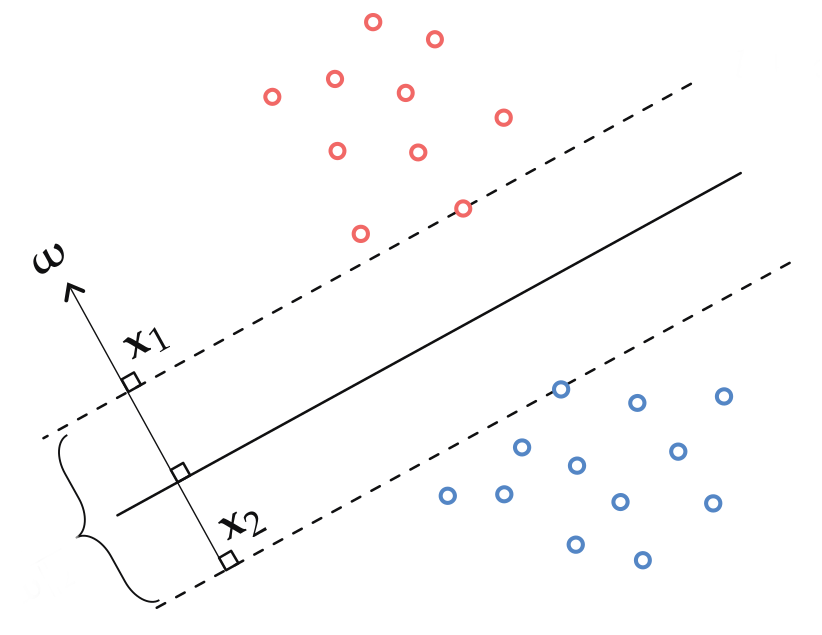
The width is given by: \[\begin{align*} \mathbf{x_1^T w} - \mathbf{x_2^T w} &= 2 \\ (\mathbf{x_1}-\mathbf{x_2})^T\mathbf{w} &= 2\\ ||\mathbf{x_1} - \mathbf{x_2}||_2||\mathbf{w}||_2 \cos(\theta) &= 2 \\ \therefore ||\mathbf{x_1} - \mathbf{x_2}||_2 &= \frac{2}{||\mathbf{w}||_2} \end{align*}\]
Hence, our objective can be restated as: \[ \max_{\mathbf{w}} \frac{2}{||\mathbf{w}||^2_2} \quad \text{subject to} \quad (\mathbf{w^T x_i})y_i \ge 1 \quad \text{for all } i \]
Equivalently, we can frame it as a minimization problem: \[ \min_{\mathbf{w}} \frac{1}{2}||\mathbf{w}||^2_2 \quad \text{subject to} \quad (\mathbf{w^T x_i})y_i \ge 1 \quad \text{for all } i \]
In summary, finding the separating hyperplane with the maximum margin is equivalent to finding the one with the smallest possible normal vector \(\mathbf{w}\).
Constrained Optimization and Dual Problem in Lagrange Multipliers
In the realm of constrained optimization, we encounter problems formulated as follows: \[\begin{align*} \min_{\mathbf{w}} f(\mathbf{w}) \\ s.t. \ g(\mathbf{w}) \le 0 \end{align*}\]
To tackle such problems effectively, the method of Lagrange Multipliers comes into play. Lagrange multipliers are instrumental in solving constrained optimization problems by identifying optimal values of an objective function while adhering to a set of constraints. In this method, the constraints are seamlessly integrated into the objective function through the introduction of auxiliary variables known as Lagrange multipliers.
Lagrange Function
For the optimization problem described above, the Lagrange function, denoted as \(\mathcal{L}(\mathbf{w}, \boldsymbol{\alpha})\), is defined as follows: \[ \mathcal{L}(\mathbf{w}, \boldsymbol{\alpha}) = f(\mathbf{w}) + \boldsymbol{\alpha}^T g(\mathbf{w}) \quad \text{for all } \mathbf{w} \]
Here, \(\boldsymbol{\alpha}\) is a vector of Lagrange multipliers, constrained to be non-negative (\(\boldsymbol{\alpha} \ge \mathbf{0}\)).
Maximizing the Lagrange function with respect to \(\boldsymbol{\alpha}\) leads us to the following formulation: \[\begin{align*} \max_{\boldsymbol{\alpha} \ge \mathbf{0}} \mathcal{L}(\mathbf{w}, \boldsymbol{\alpha}) &= \max_{\boldsymbol{\alpha} \ge \mathbf{0}} \left(f(\mathbf{w}) + \boldsymbol{\alpha}^T g(\mathbf{w})\right) \\ &= \begin{cases} \infty & \text{if } g(\mathbf{w}) > \mathbf{0} \\ f(\mathbf{w}) & \text{if } g(\mathbf{w}) \le \mathbf{0} \end{cases} \end{align*}\]
Since the Lagrange function is equivalent to \(f(\mathbf{w})\) when \(g(\mathbf{w}) \le \mathbf{0}\), we can rewrite our original problem as follows: \[\begin{align*} \min_{\mathbf{w}} f(\mathbf{w}) &= \min_{\mathbf{w}} \left[\max_{\boldsymbol{\alpha} \ge \mathbf{0}} \mathcal{L}(\mathbf{w}, \boldsymbol{\alpha})\right] \\ &= \min_{\mathbf{w}} \left[\max_{\boldsymbol{\alpha} \ge \mathbf{0}} \left(f(\mathbf{w}) + \boldsymbol{\alpha}^T g(\mathbf{w})\right)\right] \end{align*}\]
In general, interchanging the positions of the min and max functions is not permissible unless all involved functions are convex. In our case, both \(f\) and \(g\) are convex functions, allowing us to express this as: \[ \min_{\mathbf{w}} \left[\max_{\boldsymbol{\alpha} \ge \mathbf{0}} \left(f(\mathbf{w}) + \boldsymbol{\alpha}^T g(\mathbf{w})\right)\right] \equiv \max_{\boldsymbol{\alpha} \ge \mathbf{0}} \left[\min_{\mathbf{w}} \left(f(\mathbf{w}) + \boldsymbol{\alpha}^T g(\mathbf{w})\right)\right] \]
Multiple Constraints
Now, extending our discussion to scenarios with \(m\) constraints, denoted as \(g_i(\mathbf{w}) \le \mathbf{0}\) for \(i \in [1, m]\), we can represent the problem as follows: \[\begin{align*} \min_{\mathbf{w}} f(\mathbf{w}) &\equiv \min_{\mathbf{w}} \left[\max_{\boldsymbol{\alpha} \ge \mathbf{0}} f(\mathbf{w}) + \sum _{i=1} ^m \alpha _i g_i(\mathbf{w})\right] \\ &\equiv \max_{\boldsymbol{\alpha} \ge \mathbf{0}} \left[\min_{\mathbf{w}} f(\mathbf{w}) + \sum _{i=1} ^m \alpha _i g_i(\mathbf{w})\right] \end{align*}\]
Formulating the Dual Problem
To formalize the dual problem, we start with our objective function: \[ \min_{\mathbf{w}} \frac{1}{2}||\mathbf{w}||^2_2 \quad \text{s.t.} \ (\mathbf{w}^T\mathbf{x}_i)y_i \ge 1 \quad \forall i \]
The constraints can be expressed as: \[\begin{align*} (\mathbf{w}^T\mathbf{x}_i)y_i &\ge 1 \quad \forall i \\ 1 - (\mathbf{w}^T\mathbf{x}_i)y_i &\le 0 \quad \forall i \end{align*}\]
Introducing Lagrange multipliers \(\boldsymbol{\alpha} \in \mathbb{R}^d\), we construct the Lagrange function: \[\begin{align*} \mathcal{L}(\mathbf{w}, \boldsymbol{\alpha}) &= \frac{1}{2}||\mathbf{w}||^2_2 + \sum _{i=1} ^n \alpha _i (1 - (\mathbf{w}^T\mathbf{x}_i)y_i) \end{align*}\]
Now, considering the duality principle, we arrive at: \[\begin{align*} \min_{\mathbf{w}} \max_{\boldsymbol{\alpha} \ge \mathbf{0}} \left[\frac{1}{2}||\mathbf{w}||^2_2 + \sum _{i=1} ^n \alpha _i (1 - (\mathbf{w}^T\mathbf{x}_i)y_i)\right] &\equiv \max_{\boldsymbol{\alpha} \ge \mathbf{0}} \min_{\mathbf{w}} \left[\frac{1}{2}||\mathbf{w}||^2_2 + \sum _{i=1} ^n \alpha _i (1 - (\mathbf{w}^T\mathbf{x}_i)y_i)\right] \end{align*}\]
Solving for the inner function of the dual problem, we obtain: \[\begin{align*} \mathbf{w}_{\boldsymbol{\alpha}}^* - \sum _{i=1} ^n \alpha _i \mathbf{x}_i y_i = 0 \end{align*}\]
This leads to a vectorized form: \[ \mathbf{w}_{\boldsymbol{\alpha}}^* = \mathbf{XY}\boldsymbol{\alpha} \quad \ldots[1] \]
Here, \(\mathbf{X} \in \mathbb{R}^{d \times n}\) represents the dataset, \(\mathbf{Y} \in \mathbb{R}^{n \times n}\) is a diagonal matrix with label values on its diagonals, and \(\boldsymbol{\alpha} \in \mathbb{R}^{n}\).
Rewriting the outer dual function, we get, \[\begin{align*} &\max_{\boldsymbol{\alpha} \ge \mathbf{0}} \left[ \frac{1}{2}||\mathbf{w}||^2_2 + \sum _{i=1} ^n \alpha _i (1 - (\mathbf{w}^T\mathbf{x}_i)y_i) \right] \\ &= \max_{\boldsymbol{\alpha} \ge \mathbf{0}} \left[ \frac{1}{2}\mathbf{w}^T\mathbf{w} + \sum _{i=1} ^n \alpha_i - \mathbf{w}^T\mathbf{XY}\boldsymbol{\alpha} \right] \\ &= \max_{\boldsymbol{\alpha} \ge \mathbf{0}} \left[ \frac{1}{2}(\mathbf{XY}\boldsymbol{\alpha})^T(\mathbf{XY}\boldsymbol{\alpha}) + \sum _{i=1} ^n \alpha_i - (\mathbf{XY}\boldsymbol{\alpha})^T(\mathbf{XY}\boldsymbol{\alpha}) \right] \quad \ldots\text{from }[1] \\ &= \max_{\boldsymbol{\alpha} \ge \mathbf{0}} \left[ \sum _{i=1} ^n \alpha_i - \frac{1}{2}(\mathbf{XY}\boldsymbol{\alpha})^T(\mathbf{XY}\boldsymbol{\alpha}) \right] \\ \end{align*}\]
Observations
Dual and Primal Variables: The duality of the SVM problem manifests in the dimensions of its variables. The dual problem is characterized by \(\boldsymbol{\alpha} \ge \mathbf{0}\), residing in \(\mathbb{R}^n\), while the primal problem deals with \(\mathbf{w}\) in \(\mathbb{R}^d\).
Simplicity of Dual Problem: Solving the dual problem is often considered “easier” compared to the primal problem.
Kernelization Potential: The dual problem’s dependence on \(\mathbf{X}^T\mathbf{X}\) opens the door for kernelization techniques.
Let’s now examine the equation: \[ \mathbf{w}^* = \sum _{i=1} ^n \alpha _i \mathbf{x}_i y_i \]
Observations on the Equation
Interpreting \(\mathbf{w}^*\): The optimal \(\mathbf{w}^*\) emerges as a linear combination of data points, where each data point’s significance is determined by the corresponding Lagrange multiplier \(\alpha_i\).
Varying Importance: Consequently, some data points exert greater influence on \(\mathbf{w}^*\) than others.
Support Vector Machine (SVM)
Duality Revisited
Revisiting the Lagrangian function: \[ \min_{\mathbf{w}} \left [\max_{\boldsymbol{\alpha} \ge \mathbf{0}} f(\mathbf{w}) + \boldsymbol{\alpha}^T g(\mathbf{w}) \right ] \equiv \max_{\boldsymbol{\alpha} \ge \mathbf{0}} \left [ \min_{\mathbf{w}} f(\mathbf{w}) + \boldsymbol{\alpha}^T g(\mathbf{w}) \right ] \]
Here, the primal function is on the left-hand side, and the dual function is on the right. The solutions for the primal and dual functions are denoted as \(\mathbf{w}^∗\) and \(\boldsymbol{\alpha}^*\), respectively. When these solutions are substituted into the equation, we obtain: \[ \max_{\boldsymbol{\alpha} \ge \mathbf{0}} f(\mathbf{w}^*) + \boldsymbol{\alpha}^T g(\mathbf{w}^*) = \min_{\mathbf{w}} f(\mathbf{w}) + \boldsymbol{\alpha}^{*T} g(\mathbf{w}) \]
Given that \(g(\mathbf{w}^*) \le \mathbf{0}\), the left-hand side simplifies to \(f(\mathbf{w}^*)\): \[ f(\mathbf{w}^*) = \min_{\mathbf{w}} f(\mathbf{w}) + \boldsymbol{\alpha}^{*T} g(\mathbf{w}) \]
Substituting \(\mathbf{w}^*\) for \(\mathbf{w}\) in the right-hand side yields a new right-hand side that is greater than or equal to the current one: \[ f(\mathbf{w}^*) \le f(\mathbf{w}^*) + \boldsymbol{\alpha}^{*T} g(\mathbf{w}^*) \]
Hence, we can infer: \[ \boldsymbol{\alpha}^{*T} g(\mathbf{w}^*) \ge \mathbf{0} \]
However, considering the constraints, where \(\boldsymbol{\alpha}^{*} \ge \mathbf{0}\) and \(g(\mathbf{w}^*)\le \mathbf{0}\), we arrive at: \[ \boldsymbol{\alpha}^{*T} g(\mathbf{w}^*) \le \mathbf{0} \]
From this, we deduce: \[ \boldsymbol{\alpha}^{*T} g(\mathbf{w}^*) = \mathbf{0} \]
Extending this equation for multiple constraints, we obtain: \[ \alpha_i^{*} g(w^*_i) = 0 \quad \forall i \]
Hence, if one of the two values is greater than zero, the other must be zero. Considering \(g(\mathbf{w}^*) = 1-(\mathbf{w}^T\mathbf{x}_i)y_i\), we can express this as: \[ \alpha_i^{*} (1-(\mathbf{w}^T\mathbf{x}_i)y_i) = 0 \quad \forall i \]
Importantly, when \(\alpha_i > \mathbf{0}\), we deduce: \[ (\mathbf{w}^T\mathbf{x}_i)y_i = 1 \]
This implies that the \(i^{th}\) data point resides on the “Supporting” hyperplane and significantly contributes to the determination of \(\mathbf{w}^*\).
Consequently, data points with \(\alpha_i > \mathbf{0}\) earn the title of Support Vectors, and this algorithm is known as the Support Vector Machine (SVM).
Definition of Support Vector Machines (SVMs)
Support Vector Machines (SVMs) stand as a category of supervised learning algorithms designed for classification and regression analysis. SVMs aim to identify the optimal hyperplane that maximizes the margin between data points from different classes. In scenarios where data is not linearly separable, SVMs employ kernel functions to map the data into a higher-dimensional space where a linear decision boundary can effectively segregate the classes.
Insight: \(\mathbf{w}^*\) represents a sparse linear combination of data points.
Hard-Margin SVM Algorithm
The Hard-Margin SVM algorithm is applicable only when the dataset is linearly separable with a margin parameter \(\gamma > 0\). Its key steps include:
Direct or Kernelized Calculation of Q: Compute the matrix \(Q=\mathbf{X}^T\mathbf{X}\) directly or using a kernel, based on the dataset.
Gradient Descent: Employ the gradient of the dual formula, \(\boldsymbol{\alpha}^T\mathbf{1} - \frac{1}{2}\boldsymbol{\alpha}^T\mathbf{Y}^T Q\mathbf{Y}\boldsymbol{\alpha}\), in a gradient descent algorithm to iteratively find a satisfactory set of Lagrange multipliers \(\boldsymbol{\alpha}\). Initialize \(\boldsymbol{\alpha}\) as a zero vector in \(\mathbb{R}^n_+\).
Prediction: For prediction, follow these formulas:
- For non-kernelized SVM:
\(\textbf{label}(\mathbf{x}_{\text{test}}) = \text{sign}( \mathbf{w}^T\mathbf{x}_{\text{test}}) = \text{sign}\left(\displaystyle\sum _{i=1} ^n \alpha _i y_i(\mathbf{x}_i^T\mathbf{x}_{\text{test}})\right)\)
- For kernelized SVM:
\(\textbf{label}(\mathbf{x}_{\text{test}}) = \text{sign}(\mathbf{w}^T\boldsymbol{\phi}(\mathbf{x}_{\text{test}})) = \text{sign}\left(\displaystyle\sum _{i=1} ^n \alpha _i y_i k(\mathbf{x}_i^T\mathbf{x}_{\text{test}})\right)\)
Soft-Margin SVM
Soft-Margin SVM extends the standard SVM algorithm to accommodate some misclassifications in the training data. This extension is particularly useful when dealing with non-linearly separable data. It introduces a regularization parameter (\(C\)) to control the balance between maximizing the margin and allowing for misclassifications.
The primal formulation for this extension can be expressed as: \[ \min_{\mathbf{w}, \boldsymbol{\epsilon}} \frac{1}{2}||\mathbf{w}||^2_2 + C\sum _{i=1} ^n\epsilon_i \quad s.t. \quad (\mathbf{w}^T\mathbf{x}_i)y_i + \epsilon_i \ge 1;\quad \epsilon_i \ge 0\quad \forall i \]
Here, \(C\) serves as a hyperparameter governing the trade-off between maximizing the margin and minimizing misclassifications. The additional variable \(\epsilon_i\) represents the adjustment needed to satisfy the constraints.