Probabilistic PCA

Colab Link: Click here!

import numpy as np
import matplotlib.pyplot as plt
from scipy.stats import multivariate_normal
from scipy.stats import norm
import seaborn as sns

rng = np.random.default_rng(seed=12)

PCA Review

Use cases	Methodology
Analyze data and extract variables with similar concepts (principal components)	Maximizing variance of the projected dataset \mathbf{X}
Project the data onto a lower dimensional space	Represent \mathbf{X} in a different space spanned by an orthonormal basis \mathbf{W} - where columns of \mathbf{W} correspond to the eigenvectors of \mathbf{X}
Principal components that capture greater variance (equivalent to corresponding eigenvalue) are considered more important	Considering likelihood to be the reconstruction error and calculating Maximum-Likelihood estimators

X = rng.multivariate_normal((2, 3), [[5, 3], [3, 3]], size=20)

# Perform PCA on X

plt.figure(figsize=(12, 5))

X_mean = X.mean(axis=0)

X_centered = X - X_mean
cov_X = np.cov(X_centered.T)
eig_val, eig_vec = np.linalg.eigh(cov_X)
pc_vec = eig_vec[:,-1] / eig_vec[:,-1][0]
x_range = np.array([-5, 6])

plt.subplot(1, 2, 1)
plt.scatter(X[:, 0], X[:, 1], s=10);
plt.plot(x_range + X_mean[0], x_range * pc_vec[1] + X_mean[1], color='black')
plt.axis('scaled')

plt.subplot(1, 2, 2)
plt.scatter(X[:, 0], X[:, 1], s=10);
X_proj = np.array([i * eig_vec[:, -1] + X_mean for i in X_centered @ eig_vec[:, -1]])
plt.scatter(X_proj[:, 0], X_proj[:, 1], s=20, color='red');
plt.plot(x_range + X_mean[0], x_range * pc_vec[1] + X_mean[1], color='black')
plt.axis('scaled')

plt.show()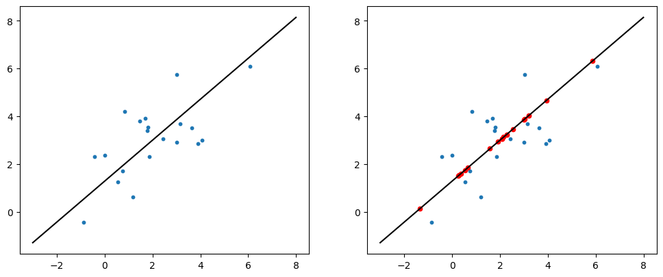

Probabilistic PCA

Reformulation of PCA in a probabilistic form, brings several advantages over conventional PCA:

• An EM algorithm for PCA can be derived that is efficient when only a few leading eigenvectors are needed, and it avoids the need to evaluate the data covariance matrix.
• The combination of a probabilistic model and EM can handle missing values in the dataset.
• Mixtures of probabilistic PCA models can be systematically formulated and trained using the EM algorithm.
• The existence of a likelihood function allows for direct comparison with other probabilistic density models. For example, if there is an outlier-like point that is far away from the training set however is close to a principal component, then conventional PCA will assign a lower reconstruction cost.
• The probabilistic PCA model can be used generatively to produce samples from the distribution.

Generative Modelling

In generative modelling, we try to induce a latent variable \mathbf{Z} of a lower dimension, which will help represent high-dimensional variable \mathbf{X}.

In the context of PCA, \mathbf{Z} will represent the mappings of \mathbf{X} on a lower dimensional subspace, which corresponds to the principal subspace.

So how do we introduce \mathbf{Z}?

A generative story

Let L and D be the dimension of the latent space \mathbf{Z} and data space \mathbf{X} respectively.

The following steps are followed to generate a new sample \mathbf{x}:

• Sample \mathbf{z} from the prior defined as p(\mathbf{z}) = \mathcal{N}(\mathbf{z}|0, \mathbf{I})
• Further, sample \mathbf{x} using \mathbf{z} from the conditional distribution p(\mathbf{x}|\mathbf{z}) = \mathcal{N}(\mathbf{x}|\mathbf{W}\mathbf{z}+\mathbf{\mu}, σ^2\mathbf{I})

We require \mathbf{W} to span a linear subspace, corresponding to the principal subspace of \mathbf{X}.

We illustrate this below for the simple case where D=2, L=1. We obtain parameter values for the distribution from PCA performed above in the notebook. We see that the dataset can effectively be regenerated after estimating parameters of our model.

from IPython.display import HTML
from matplotlib import animation
import warnings 

warnings.filterwarnings("ignore")


M, N = np.mgrid[-6:10:0.1, -6:10:0.1]
grid = np.dstack((M, N))

x = np.linspace(-4, 4)
z = rng.standard_normal()
w = pc_vec/np.sqrt(pc_vec.T@pc_vec)
n, d = X.shape

mu = X.mean(axis=0)
s2 = eig_val[0]
X_gen = []

theta = np.linspace(0, 2*np.pi, 1000)
circle = np.c_[np.cos(theta), np.sin(theta)]

fig, (ax1, ax2, ax3) = plt.subplots(1, 3, figsize=(10, 100/36))
norm_pdf = ax1.plot(x, norm.pdf(x, 0, 1))
ax2_line = ax2.plot(x_range + X_mean[0], x_range * pc_vec[1] + X_mean[1], color='black')

# zeroth frame - pdf, line graph
default = norm_pdf + ax2_line
artists = [list(default)]

for _ in range(15):
  # sampling x
  x_mean = np.expand_dims(z*w+mu, -1).T
  x = rng.multivariate_normal(z*w+mu, cov=s2*np.eye(2))

  frame = list(default)

  # first frame - sample z
  z = rng.standard_normal()
  frame.append(ax1.scatter(z, 0, marker='x', color='red'))

  artists.append(list(frame))

  # second frame - visualize p(x|z)
  frame += ax2.plot((x_mean + 0.5*s2*circle)[:, 0], (x_mean + 0.5*s2*circle)[:, 1], color='red')
  frame += ax2.plot((x_mean + 1*s2*circle)[:, 0], (x_mean + 1*s2*circle)[:, 1], color='red')
  frame += ax2.plot((x_mean + 1.5*s2*circle)[:, 0], (x_mean + 1.5*s2*circle)[:, 1], color='red')

  artists.append(list(frame))

  # third frame - sample x, show collection
  frame.append(ax2.scatter(x[0], x[1], color='orange', marker='x'))
  new_point_plot = ax3.scatter(x[0], x[1], color='orange', s=10)
  frame.append(new_point_plot)
  artists.append(list(frame))

  # preserve new point by incrementing default collection
  default.append(new_point_plot)

else:
  frame = list(default)
  probability_grid = multivariate_normal(X.mean(axis=0), w@w.T + s2*np.eye(d)).pdf(grid)
  frame += ax2.contour(M, N, probability_grid).collections
  frame += ax3.contour(M, N, probability_grid).collections

artists.append(list(frame))

plt.close()
ax3.sharex(ax2);
ax3.sharey(ax2);
ax2.axis('scaled');ax3.axis('scaled');

ax1.title.set_text('Sampling z from latent space')
ax2.title.set_text('Sampling x from data space')
ax3.title.set_text('Collection of sampled points')

anim = animation.ArtistAnimation(fig, artists, interval=600, repeat=False, blit=False);
HTML(anim.to_jshtml())

Once Loop Reflect

In the final frame of the above animation, we see that the genrative story effectively reduces to the sampling of \mathbf{X} from the following distribution: \begin{alignat}{2} && p(\mathbf{x}) &= \int{p(\mathbf{x}|\mathbf{z})p(\mathbf{z}) d\mathbf{z}} \\ && &= \mathcal{N}(\mathbf{x}|\mathbf{\mu}, \mathbf{W}\mathbf{W}^T + σ^2\mathbf{I}) \end{alignat}

The above derivation is easy by noting that p(\mathbf{x}) is gaussian. So one can just find the mean and covariance:

\begin{alignat}{2} && \mathbb{E}[\mathbf{x}] &= \mathbb{E}[\mathbf{Wz + \mu + ϵ}] = \mathbf{\mu} \\ && \mathrm{cov}[\mathbf{x}] &= \mathbb{E}[(\mathbf{Wz + ϵ})(\mathbf{Wz + ϵ})^T] \\ && &= \mathbb{E}[\mathbf{Wzz^TW^T}] + \mathbb{E}[\mathbf{ϵϵ^T}] = \mathbf{WW^T} + σ^2\mathbf{I} \end{alignat}

EM for Probablistic PCA

The data log-likelihood of our model can be written as follows:

\ln p\left(\mathbf{X}, \mathbf{Z} \mid \boldsymbol{\mu}, \mathbf{W}, \sigma^2\right)=\sum_{n=1}^N\left\{\ln p\left(\mathbf{x}_n \mid \mathbf{z}_n\right)+\ln p\left(\mathbf{z}_n\right)\right\}

Maximizing the above function is a little complex, but closed-form solutions do exist for the ML estimators. We will, however, follow an iterative approach by formulating an EM Algorithm:

E-step

The E-step estimates the conditional distribution of the hidden variables \mathbf{Z} given the data \mathbf{X} and the current values of the model parameters \mathbf{W, σ^2} (note that ML estimate of \mathbf{\mu} is simply the sample mean \mathbf{\overline{X}}, so it can simly be mean-centered in the preprocessing step)

\begin{alignat}{2} Σ_\mathbf{Z} &= σ^2(σ^2\mathbf{I}+\mathbf{W^TW})^{-1}, \\ \mathbf{Z} &= \frac{1}{σ^2}Σ_\mathbf{Z}\mathbf{W}^T\mathbf{Y} \end{alignat}

M-step

The M-Step re-estimates the model paramters as

\begin{aligned} \mathbf{W} & =\mathbf{Y} {\mathbf{Z}}^{\mathrm{T}}\left({\mathbf{Z Z}}^{\mathrm{T}}+n \Sigma_{\mathbf{Z}}\right)^{-1}, \\ σ^2 & =\frac{1}{ND} \sum_{i=1}^d \sum_{j=1}^n\left(y_{i j}-\mathbf{w}_i^{\mathrm{T}} {\mathbf{z}}_j\right)^2+\frac{1}{d} \operatorname{tr}\left(\mathbf{W} \Sigma_{\mathbf{Z}} \mathbf{W}^{\mathrm{T}}\right) . \end{aligned}

# Initialization
X_ = (X-X.mean(axis=0)).T
W = np.array([[1, -1]]).T
s2 = 0.1

artists = []
fig, ax = plt.subplots(dpi=150)
ax.sharex(ax2)
ax.sharey(ax2)

default = [ax.scatter(X[:, 0], X[:, 1], s=10)]

for _ in range(7):
  frame = list(default)
  pc = W.T[0]/W.T[0][0]
  probability_grid = multivariate_normal(X.mean(axis=0), W@W.T + s2*np.eye(d)).pdf(grid)

  frame += ax.contour(M, N, probability_grid).collections
  frame +=  ax.plot(x_range + X_mean[0], x_range * pc[1] + X_mean[1], color='black')

  # E-step
  cov_Z = s2*np.linalg.inv(s2*np.eye(W.shape[1]) + W.T@W)
  Z = cov_Z*W.T@X_ / s2

  # M-step
  W = X_@Z.T@np.linalg.inv(Z@Z.T + X_.shape[1]*cov_Z)
  s2 = ((X_-W@Z)**2).sum()/(n*d) + np.trace(W@cov_Z@W.T)/d
  artists.append(frame)

plt.close()
anim = animation.ArtistAnimation(fig, artists, interval=500, repeat=False, blit=False);
HTML(anim.to_jshtml())

Once Loop Reflect

In the above animation, the updates made to p(\mathbf{x}) after each M-step is shown.

EM for Standard PCA

In the above probabilistic formulation, if we take the limit σ^2→0 we end up again in standard PCA. However, the EM algortihm simplifies nicely, giving the following elegant algorithm:

\begin{aligned} \text{E-Step: }\\ \mathbf{Z} &= (\mathbf{W^TW})^{-1}\mathbf{W}^T\mathbf{X}\\ \text{M-Step: }\\ \mathbf{W} &= \mathbf{X}^T\mathbf{Z}^T(\mathbf{ZZ}^T)^{-1} \end{aligned}

• The E-Step is just an orthogonal projection of the data.
• The M-Step corresponds to a multi-output linear regression where \mathbf{Z} from E-Step acts as the features, and \mathbf{X} the labels.

# Initialization
X_ = (X-X.mean(axis=0)).T
W = np.array([[1, -1]]).T
s2 = 0.1

M, N = np.mgrid[-6:10:0.1, -6:10:0.1]
grid = np.dstack((M, N))

d, n = X_.shape

artists = []
fig, ax = plt.subplots(dpi=150)

default = [ax.scatter(X[:, 0], X[:, 1], s=10)]

for _ in range(5):
  frame = list(default)
  pc = W.T[0]/W.T[0][0]
  w_ortho = pc/np.linalg.norm(pc)
  ortho_points = np.array([i * w_ortho for i in X_.T @ w_ortho])

  frame +=  ax.plot(x_range + X_mean[0], x_range * pc[1] + X_mean[1], color='black')
  for i, j in zip(X, ortho_points):
    frame += ax.plot([i[0], j[0]+X_mean[0]], [i[1], j[1]+X_mean[1]], color='red')

  artists.append(frame)
  frame = list(default)

  # E-step
  Z = np.linalg.inv(W.T@W)*W.T@X_
  # M-step
  W = X_@Z.T@np.linalg.inv(Z@Z.T)

  pc = W.T[0]/W.T[0][0]
  w_ortho_new = pc/np.linalg.norm(pc)
  alpha = np.arccos(w_ortho.T@w_ortho_new)

  rot = np.array([[np.cos(alpha), np.sin(alpha)], [-1*np.sin(alpha), np.cos(alpha)]])
  released_points = ortho_points@rot

  frame += ax.plot(x_range + X_mean[0], x_range * pc[1] + X_mean[1], color='black')
  for i, j in zip(X, released_points):
    frame += ax.plot([i[0], j[0]+X_mean[0]], [i[1], j[1]+X_mean[1]], color='red')

  artists.append(frame)

ax.axis('equal')
plt.close()
anim = animation.ArtistAnimation(fig, artists, interval=500, repeat=False, blit=False);
HTML(anim.to_jshtml())

Once Loop Reflect

The above animation also illustrates a simple physical analogy for PCA using EM, for the case when D=2 and L=1: - In the E-step, we attach the data to a rigid fixed rod with direction \mathbf{w} orthogonally using a spring that obeys Hooke’s law - In the M-step, keeping the attachments fixed, we release the rod and allow it to minimize spring energy.

The alternating of the above 2 steps corresponds to the EM algorithm for conventional PCA.