Inductive Bias in Decision Trees and K-Nearest Neighbors

Slides: Click here!

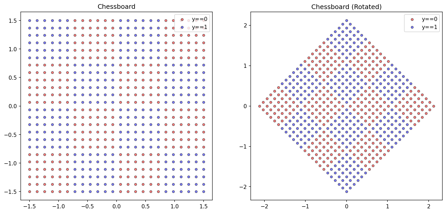
Construct a checkerboard Dataset

from matplotlib import pyplot as plt
import numpy as np

plt.rcParams['figure.figsize'] = (14, 6.3)
plt.rcParams['figure.dpi'] = 150
plt.rcParams['lines.markersize'] = 4.2

X, y = [], []
r, c = -1, -1
d = 4
n = 6
for i in np.linspace(0, 3, num=d*n):
  r += 1
  for j in np.linspace(0, 3, num=d*n):
    c += 1
    X.append([i, j])
    y.append(int(bool((r//n)%2) and not bool((c//n)%2) or not bool((r//n)%2) and bool((c//n)%2)))

X = np.array(X)
X -= np.mean(X, axis=0)
y = np.array(y)

r = np.pi/4
rotate = np.array([[np.cos(r), np.sin(r)], [np.sin(r), -np.cos(r)]])
X_rotated = X@rotate

fig, (ax1, ax2) = plt.subplots(1, 2)
ax1.scatter(X[:, 0][y==0], X[:, 1][y==0], color='red', label='y==0', alpha=0.5, edgecolor='k')
ax1.scatter(X[:, 0][y==1], X[:, 1][y==1], color='blue', label='y==1', alpha=0.5, edgecolor='k')
ax1.legend()
ax1.set_title('Chessboard')

ax2.scatter(X_rotated[:, 0][y==0], X_rotated[:, 1][y==0], color='red', label='y==0', alpha=0.5, edgecolor='k')
ax2.scatter(X_rotated[:, 0][y==1], X_rotated[:, 1][y==1], color='blue', label='y==1', alpha=0.5, edgecolor='k')
ax2.legend()
ax2.set_title('Chessboard (Rotated)')

Text(0.5, 1.0, 'Chessboard (Rotated)')

Decision Trees

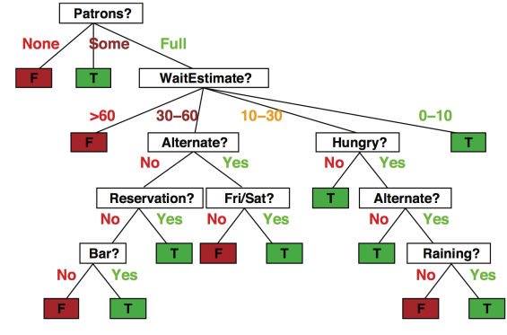
Popular representation for interpretable classifiers; even among humans!

Example: I’ve just arrived at a restaurant. Should I stay (wait for a table) or go elsewhere?

One may choose to use the following set of rules to make their decision:

source: ai.berkeley.edu

Decision trees: - Have a simple Design - Interpretable - Easy to implement - Good performance in practice

Note that splits happen individually at the feature level - corresponds to splits parallel to a feature axis - Inductive bias

Inductive bias

Anything which makes the algorithm learn one pattern instead of another pattern.

Decision trees use a step-function collection for classification; but these step functions utilize one feature/variable only. Is this phenomenon sensitive to the nature of the dataset?

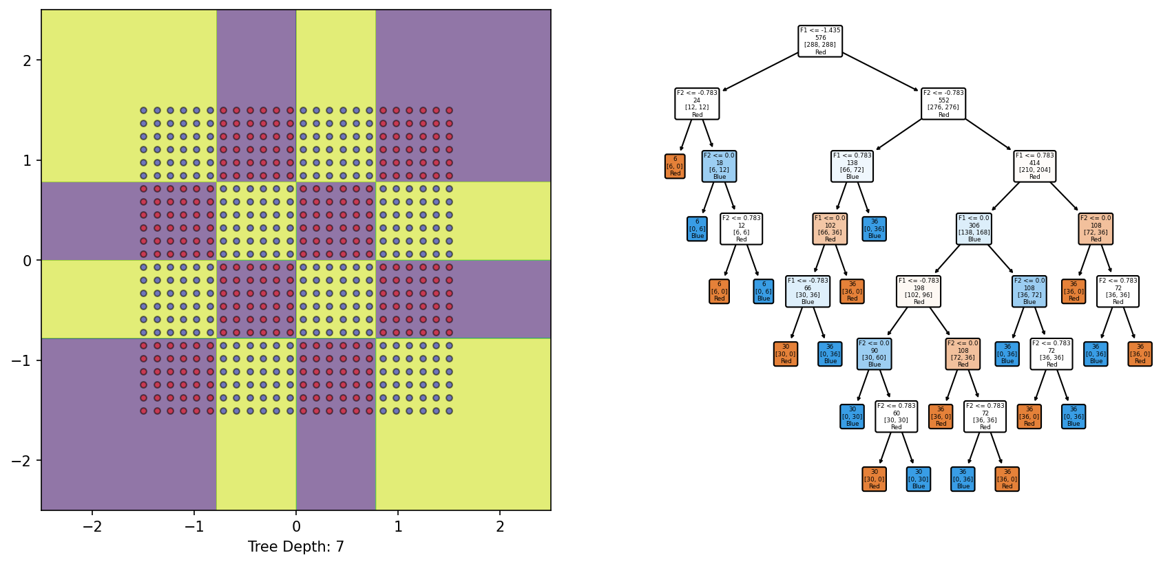
from sklearn.inspection import DecisionBoundaryDisplay
from sklearn.tree import DecisionTreeClassifier
from sklearn.tree import plot_tree

DTree = DecisionTreeClassifier()
DTree.fit(X, y)

fig, (ax1, ax2) = plt.subplots(1, 2)

disp = DecisionBoundaryDisplay.from_estimator(DTree, X, response_method="predict", grid_resolution=1000, alpha=0.6, ax = ax1)
disp.ax_.scatter(X[:, 0][y==0], X[:, 1][y==0], color='red', label='y==0', edgecolor='k', alpha=0.5)
disp.ax_.scatter(X[:, 0][y==1], X[:, 1][y==1], color='blue', label='y==1', edgecolor='k', alpha=0.5)
disp.ax_.set_xlabel(f'Tree Depth: {DTree.get_depth()}');

plot_tree(DTree, label='none', filled=True, feature_names=['F1', 'F2'], class_names=['Red', 'Blue'], node_ids=False, rounded=True, impurity=False, ax=ax2);

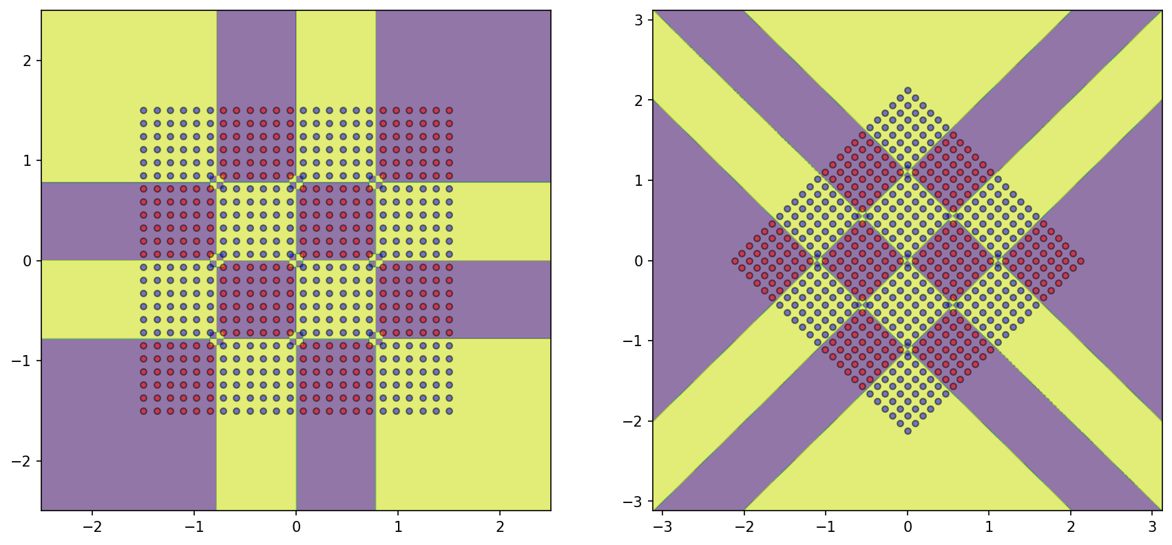
The 4x4 checkerboard dataset with alternating classes requires a tree of depth=7 to capture its structure respectively.

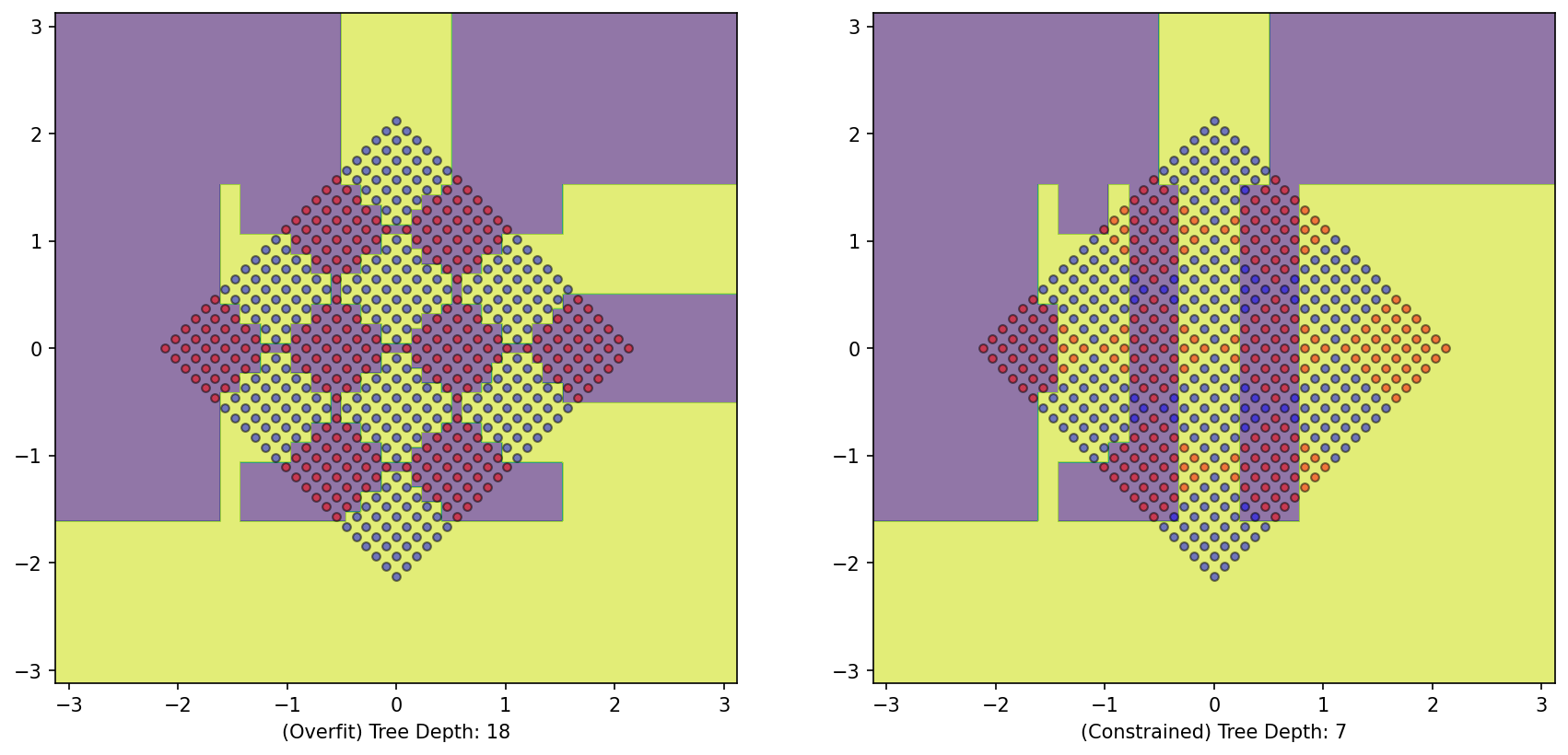
But what will happen if we try to train a tree on the rotated variant of this dataset?

fig, (ax1, ax2) = plt.subplots(1, 2)

DTree_rotated = DecisionTreeClassifier()
DTree_rotated.fit(X_rotated, y)

disp = DecisionBoundaryDisplay.from_estimator(DTree_rotated, X_rotated, response_method="predict", grid_resolution=1000, alpha=0.6, ax=ax1)
disp.ax_.scatter(X_rotated[:, 0][y==0], X_rotated[:, 1][y==0], color='red', label='y==0', edgecolor='k', alpha=0.5)
disp.ax_.scatter(X_rotated[:, 0][y==1], X_rotated[:, 1][y==1], color='blue', label='y==1', edgecolor='k', alpha=0.5)
disp.ax_.set_xlabel(f'(Overfit) Tree Depth: {DTree_rotated.get_depth()}')

DTree_rotated_constrained = DecisionTreeClassifier(max_depth=7)
DTree_rotated_constrained.fit(X_rotated, y)

disp = DecisionBoundaryDisplay.from_estimator(DTree_rotated_constrained, X_rotated, response_method="predict", grid_resolution=1000, alpha=0.6, ax=ax2)
disp.ax_.scatter(X_rotated[:, 0][y==0], X_rotated[:, 1][y==0], color='red', label='y==0', edgecolor='k', alpha=0.5)
disp.ax_.scatter(X_rotated[:, 0][y==1], X_rotated[:, 1][y==1], color='blue', label='y==1', edgecolor='k', alpha=0.5)
disp.ax_.set_xlabel(f'(Constrained) Tree Depth: {DTree_rotated_constrained.get_depth()}');

Oh!

The model fails to understand the generation rationale of the dataset as it suffers an inductive bias of axis-parallel splitting.

KNN

Examine the performance of KNN (with neighbors=3) on both variants of the dataset

from sklearn.neighbors import KNeighborsClassifier

fig, (ax1, ax2) = plt.subplots(1, 2)

knn = KNeighborsClassifier(n_neighbors=3)
knn.fit(X, y)

disp = DecisionBoundaryDisplay.from_estimator(knn, X, response_method="predict", grid_resolution=1000, alpha=0.6, ax=ax1)
disp.ax_.scatter(X[:, 0][y==0], X[:, 1][y==0], color='red', label='y==0', edgecolor='k', alpha=0.5)
disp.ax_.scatter(X[:, 0][y==1], X[:, 1][y==1], color='blue', label='y==1', edgecolor='k', alpha=0.5)

knn_rotated = KNeighborsClassifier(n_neighbors=3)
knn_rotated.fit(X_rotated, y)

disp = DecisionBoundaryDisplay.from_estimator(knn_rotated, X_rotated, response_method="predict", grid_resolution=1000, alpha=0.6, ax=ax2)
disp.ax_.scatter(X_rotated[:, 0][y==0], X_rotated[:, 1][y==0], color='red', label='y==0', edgecolor='k', alpha=0.5)
disp.ax_.scatter(X_rotated[:, 0][y==1], X_rotated[:, 1][y==1], color='blue', label='y==1', edgecolor='k', alpha=0.5)

<matplotlib.collections.PathCollection at 0x79d1e140c640>

The rotation performed does not impact the performance of KNN.

What is the inductive bias in KNN then?

Inductive Bias of KNN

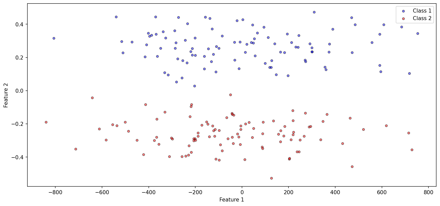
To investigate, we construct the following dataset

import numpy as np
import matplotlib.pyplot as plt

plt.rcParams['figure.figsize'] = (14, 6.3)
plt.rcParams['figure.dpi'] = 150
plt.rcParams['lines.markersize'] = 4.2

np.random.seed(0)
class1_mean = [0, 0.25]
class1_cov = [[100000, 0], [0, 0.01]]
class1_data = np.random.multivariate_normal(class1_mean, class1_cov, 100)

class2_mean = [0, -0.25]
class2_cov = [[100000, 0], [0, 0.01]]
class2_data = np.random.multivariate_normal(class2_mean, class2_cov, 100)

plt.scatter(class1_data[:, 0], class1_data[:, 1], c='b', label='Class 1', edgecolor='k', alpha=0.5)
plt.scatter(class2_data[:, 0], class2_data[:, 1], c='r', label='Class 2', edgecolor='k', alpha=0.5)
plt.xlabel('Feature 1')
plt.ylabel('Feature 2')
plt.legend()
plt.show()

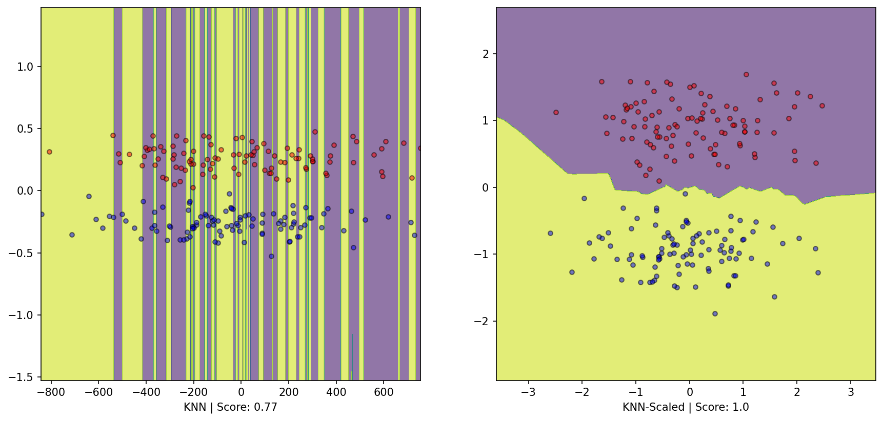
from sklearn.preprocessing import StandardScaler
from sklearn.model_selection import train_test_split

X = np.concatenate([class1_data, class2_data])
y = np.array([0 for _ in range(100)] + [1 for _ in range(100)])

X_scaled = StandardScaler().fit_transform(X)
y_scaled = y

X_train, X_test, y_train, y_test = train_test_split(X, y, test_size=0.33, random_state=42)
X_scaled_train, X_scaled_test, y_scaled_train, y_scaled_test = train_test_split(X_scaled, y, test_size=0.33, random_state=42)

knn = KNeighborsClassifier(n_neighbors=3).fit(X, y)
knn2 = KNeighborsClassifier(n_neighbors=3).fit(X_scaled, y)

fig, (ax1, ax2) = plt.subplots(1, 2)

disp = DecisionBoundaryDisplay.from_estimator(knn, X, response_method="predict", grid_resolution=1000, alpha=0.6, ax=ax1)
disp.ax_.scatter(X[:, 0][y==0], X[:, 1][y==0], color='red', label='y==0', edgecolor='k', alpha=0.5)
disp.ax_.scatter(X[:, 0][y==1], X[:, 1][y==1], color='blue', label='y==1', edgecolor='k', alpha=0.5)
disp.ax_.set_xlabel(f'KNN | Score: {knn.score(X, y)}')

disp = DecisionBoundaryDisplay.from_estimator(knn2, X_scaled, response_method="predict", grid_resolution=1000, alpha=0.6, ax=ax2)
disp.ax_.scatter(X_scaled[:, 0][y_scaled==0], X_scaled[:, 1][y_scaled==0], color='red', label='y_scaled==0', edgecolor='k', alpha=0.5)
disp.ax_.scatter(X_scaled[:, 0][y_scaled==1], X_scaled[:, 1][y_scaled==1], color='blue', label='y_scaled==1', edgecolor='k', alpha=0.5)
disp.ax_.set_xlabel(f'KNN-Scaled | Score: {knn2.score(X_scaled, y_scaled)}');

Oh!

We observe that scaling impacts the performance on the dataset. This reveals the inductive bias for KNN:

The algorithm assumes that entities belonging to a particular category should appear near each other, and those that are part of different groups should be distant.

Here even though the seperation is evident, the scaling makes this phenomenon invisible to the knn classifier; hence the model does not capture this structure in the dataset.

Perceptron

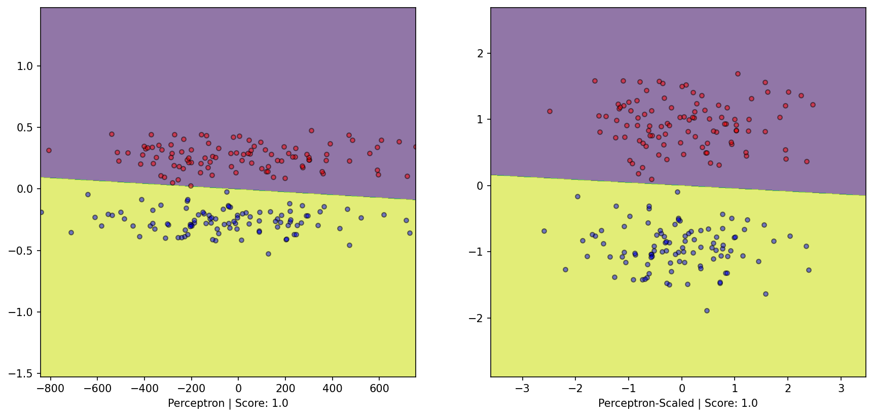
If through context we are confident that our dataset has an underlying linear seperation, we could use the Perceptron algorithm

from sklearn.linear_model import Perceptron

perceptron = Perceptron(alpha=0, max_iter=int(1e6), tol=None).fit(X, y)
perceptron_scaled = Perceptron(alpha=0, max_iter=int(1e6), tol=None).fit(X_scaled, y_scaled)

fig, (ax1, ax2) = plt.subplots(1, 2)

disp = DecisionBoundaryDisplay.from_estimator(perceptron, X, response_method="predict", grid_resolution=1000, alpha=0.6, ax=ax1)
disp.ax_.scatter(X[:, 0][y==0], X[:, 1][y==0], color='red', label='y==0', edgecolor='k', alpha=0.5)
disp.ax_.scatter(X[:, 0][y==1], X[:, 1][y==1], color='blue', label='y==1', edgecolor='k', alpha=0.5)
disp.ax_.set_xlabel(f'Perceptron | Score: {perceptron.score(X, y)}')

disp = DecisionBoundaryDisplay.from_estimator(perceptron_scaled, X_scaled, response_method="predict", grid_resolution=1000, alpha=0.6, ax=ax2)
disp.ax_.scatter(X_scaled[:, 0][y_scaled==0], X_scaled[:, 1][y_scaled==0], color='red', label='y_scaled==0', edgecolor='k', alpha=0.5)
disp.ax_.scatter(X_scaled[:, 0][y_scaled==1], X_scaled[:, 1][y_scaled==1], color='blue', label='y_scaled==1', edgecolor='k', alpha=0.5)
disp.ax_.set_xlabel(f'Perceptron-Scaled | Score: {perceptron_scaled.score(X_scaled, y_scaled)}');

Perceptron algorithm: - Is a linear Classifier - Simple update rule: on mistake; add/subtract datapoint - Shown to converge only on linearly seperable datasets with non-zero margin (radius-margin bound) - Inductive Bias due to assumption of underlying structure of data

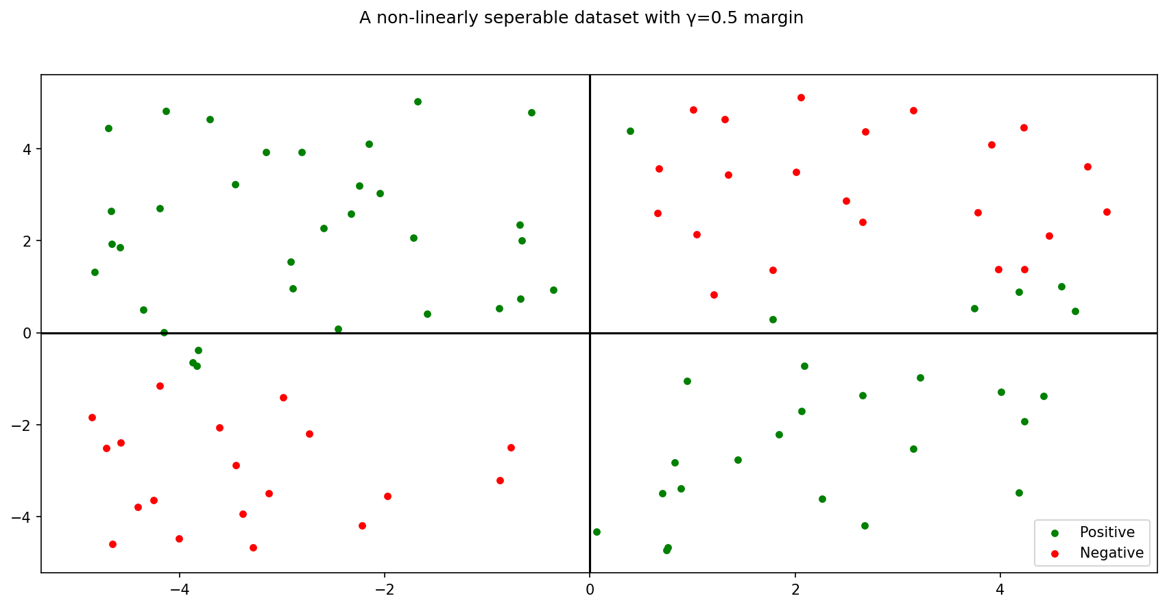
What about non-linear, say, quadratic seperability? Consider the following dataset:

np.random.seed(1)

X_ = np.random.rand(100, 2)
X_ = (X_-np.mean(X_))*10

X, y = [], []

perp = lambda i: -1*i[0]/i[1]
sign = lambda i: 2*int(i >= 0)-1

sep = lambda x: x[1]**2-8*x[1]*x[0]+2*x[0]**2

w = np.array([1, 1])/np.sqrt(2)
gamma = 0.5

for p in X_:
  d = sep(p)
  if abs(d) >= gamma:
    X.append(p)
    y.append(sign(d))

X = np.array(X)
y = np.array(y)

fig, (ax2) = plt.subplots(1, 1)
fig.suptitle(f'A non-linearly seperable dataset with γ={gamma} margin')

ax2.scatter(X[:, 0][y==1], X[:, 1][y==1], color='green', label='Positive')
ax2.scatter(X[:, 0][y!=1], X[:, 1][y!=1], color='red', label='Negative')
ax2.legend(loc='lower right')

ax2.axvline(x=0, c='black')
ax2.axhline(y=0, c='black')

plt.show()

Being Mindful of the Bias

The above dataset has a seperator corresponding to a second order function of the features.

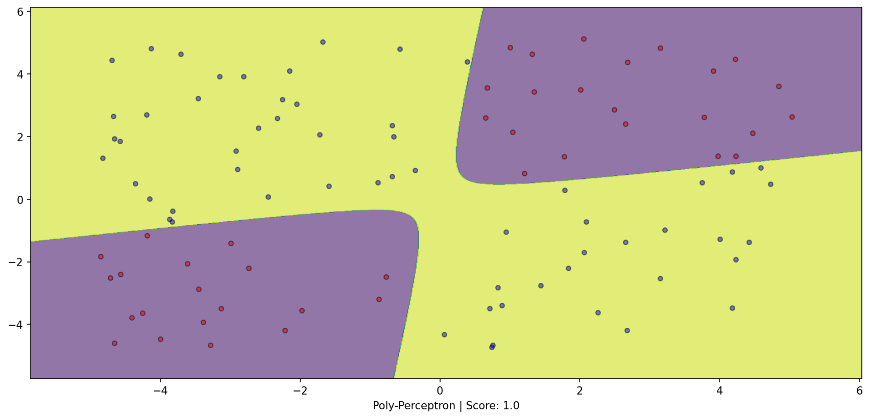
Transform the dataset and apply perceptron! Alter inductive bias to our advantage

from sklearn.pipeline import make_pipeline
from sklearn.preprocessing import PolynomialFeatures
from sklearn.linear_model import Perceptron

poly_perceptron = make_pipeline(PolynomialFeatures(2), Perceptron(alpha=0, max_iter=int(1e6), tol=None))
poly_perceptron.fit(X, y)

fig, (ax1) = plt.subplots(1, 1)
disp = DecisionBoundaryDisplay.from_estimator(poly_perceptron, X, response_method="predict", grid_resolution=1000, alpha=0.6, ax=ax1)
disp.ax_.scatter(X[:, 0][y==-1], X[:, 1][y==-1], color='red', label='y==-1', edgecolor='k', alpha=0.5)
disp.ax_.scatter(X[:, 0][y==1], X[:, 1][y==1], color='blue', label='y==1', edgecolor='k', alpha=0.5)
disp.ax_.set_xlabel(f'Poly-Perceptron | Score: {poly_perceptron.score(X, y)}');